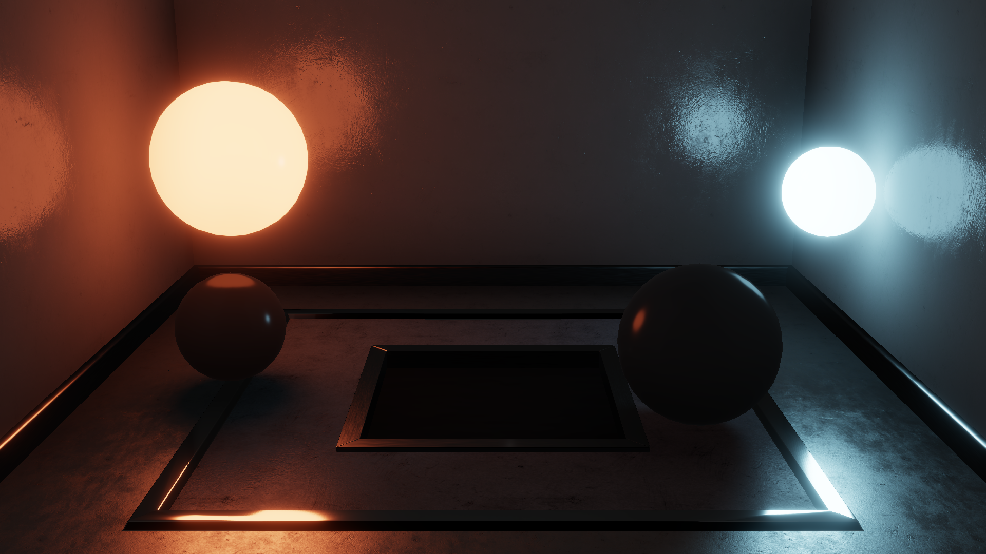
A Spherical Cap Preserving Parameterization for Spherical Distributions
Doing Stuff with Spherical Caps
| Jonathan Dupuy | Eric Heitz | Laurent Belcour |
| Unity Technologies | Unity Technologies | Unity Technologies |
A Spherical Cap Preserving Parameterization for Spherical Distributions
"Doing Stuff with Spherical Caps"
| Jonathan Dupuy | Eric Heitz | Laurent Belcour |
| Unity Technologies | Unity Technologies | Unity Technologies |
Overview
Theoretical contribution
Applied to sphere lighting
- Spherical distributions
- Analytic cap integration
- Analytic sampling
Applied to sphere lighting
- Real-time shading
- Specular occlusion
- Variance reduction

|

|

|
Overview
Theoretical contribution
Applied to sphere lighting
- Spherical distributions
- Analytic cap integration
- Analytic sampling
Applied to sphere lighting
- Real-time shading
- Specular occlusion
- Variance reduction

|

|

|
Overview
Theoretical contribution
Applied to sphere lighting
- Spherical distributions
- Analytic cap integration
- Analytic sampling
Applied to sphere lighting
- Real-time shading
- Specular occlusion
- Variance reduction

|

|

|
Overview
Theoretical contribution
Applied to sphere lighting
- Spherical distributions
- Analytic cap integration
- Analytic sampling
Applied to sphere lighting
- Real-time shading
- Specular occlusion
- Variance reduction

|

|

|
Overview
Theoretical contribution
Applied to sphere lighting
- Spherical distributions
- Analytic cap integration
- Analytic sampling
Applied to sphere lighting
- Real-time shading
- Specular occlusion
- Variance reduction

Overview
Theoretical contribution
Applied to sphere lighting
- Spherical distributions
- Analytic cap integration
- Analytic sampling
Applied to sphere lighting
- Real-time shading
- Specular occlusion
- Variance reduction

Overview
Theoretical contribution
Applied to sphere lighting
- Spherical distributions
- Analytic cap integration
- Analytic sampling
Applied to sphere lighting
- Real-time shading
- Specular occlusion
- Variance reduction
| MIS@64spp: Previous | MIS@64spp: Ours |
 |
 |
Motivation


Problem

$$\mathscr{C}$$
$$
\boxed{\;
I = \int_\mathscr{C} D(\boldsymbol{\omega}) \, d\boldsymbol{\omega}
\;}
$$
How to compute efficiently ?
Related Work

| Uniform | Clipped Uniform | Cosine |

|

|

|
| vMF (Spherical Gaussian) | Phong Lobes | ||||||
|
|
Low frequency
No closed-form
O(exponent)
Contribution

| Uniform | Clipped Uniform | Cosine |

|

|

|
| vMF (Spherical Gaussian) | Phong Lobes | ||||||
|
|
Low frequency
No closed-form
O(exponent)
| NEW Pivot Distributions | ||||
|
All frequency + closed-form + O(1)
Pivot Distributions
Pivot Distributions
Overview
Properties
- Pivot transformation
- Jacobian as PDF
Properties
- Analytic sampling
- Cap-preserving
- Analytic cap integrals
 |
+ |  |
= |  |
Pivot Distributions
Overview
Properties
- Pivot transformation
- Jacobian as PDF
Properties
- Analytic sampling
- Cap-preserving
- Analytic cap integrals
 |
+ |  |
= |  |
\begin{align}
{\color{red}\boldsymbol{\omega}}
\end{align}
Pivot Distributions
Overview
Properties
- Pivot transformation
- Jacobian as PDF
Properties
- Analytic sampling
- Cap-preserving
- Analytic cap integrals
 |
+ |  |
= |  |
\begin{align}
{\color{red}\boldsymbol{\omega}}
\mapsto
{\color{green}\boldsymbol{\omega}}
\end{align}
Pivot Distributions
Overview
Properties
- Pivot transformation
- Jacobian as PDF
Properties
- Analytic sampling
- Cap-preserving
- Analytic cap integrals
 |
+ |  |
= |  |
\begin{align}
{\color{red}\boldsymbol{\omega}}
\mapsto
{\color{green}\boldsymbol{\omega}}
&=
g({\color{red}\boldsymbol{\omega}}; {\color{RoyalBlue}\mathbf{r}_p})
\end{align}
\begin{align}
\Rightarrow
{\color{red}\boldsymbol{\omega}}
&=
g({\color{green}\boldsymbol{\omega}}; {\color{RoyalBlue}\mathbf{r}_p})
\end{align}
Pivot Distributions
Overview
Properties
- Pivot transformation
- Jacobian as PDF
Properties
- Analytic sampling
- Cap-preserving
- Analytic cap integrals
 |
+ |  |
= |  |
\begin{align}
{\color{red}\boldsymbol{\omega}}
\mapsto
{\color{green}\boldsymbol{\omega}}
&=
g({\color{red}\boldsymbol{\omega}}; {\color{RoyalBlue}\mathbf{r}_p})
\end{align}
\begin{align}
\Rightarrow
{\color{red}\boldsymbol{\omega}}
&=
g({\color{green}\boldsymbol{\omega}}; {\color{RoyalBlue}\mathbf{r}_p})
\end{align}
$$D_\textrm{std}({\color{red}\boldsymbol{\omega}})$$
\begin{align}
D({\color{red}\boldsymbol{\omega}}; {\color{RoyalBlue}\mathbf{r}_p})
=
D_\textrm{std}({\color{green}\boldsymbol{\omega}})
\frac{
d {\color{green}\boldsymbol{\omega}}
}{
d {\color{red}\boldsymbol{\omega}}
}
\end{align}
Pivot Distributions
Overview
Properties
- Pivot transformation
- Jacobian as PDF
Properties
- Analytic sampling
- Cap-preserving
- Analytic cap integrals
 |
+ |  |
= |  |
\begin{align}
{\color{red}\boldsymbol{\omega}}
\mapsto
{\color{green}\boldsymbol{\omega}}
&=
g({\color{red}\boldsymbol{\omega}}; {\color{RoyalBlue}\mathbf{r}_p})
\end{align}
\begin{align}
\Rightarrow
{\color{red}\boldsymbol{\omega}}
&=
g({\color{green}\boldsymbol{\omega}}; {\color{RoyalBlue}\mathbf{r}_p})
\end{align}
$$D_\textrm{std}({\color{red}\boldsymbol{\omega}})$$
\begin{align}
D({\color{red}\boldsymbol{\omega}}; {\color{RoyalBlue}\mathbf{r}_p})
=
D_\textrm{std}({\color{green}\boldsymbol{\omega}})
\frac{
d {\color{green}\boldsymbol{\omega}}
}{
d {\color{red}\boldsymbol{\omega}}
}
\end{align}
Pivot Distributions
Overview
Properties
- Pivot transformation
- Jacobian as PDF
Properties
- Analytic sampling
- Cap-preserving
- Analytic cap integrals
 |
+ |  |
= |  |
\begin{align}
{\color{red}\boldsymbol{\omega}}
\mapsto
{\color{green}\boldsymbol{\omega}}
&=
g({\color{red}\boldsymbol{\omega}}; {\color{RoyalBlue}\mathbf{r}_p})
\end{align}
\begin{align}
\Rightarrow
{\color{red}\boldsymbol{\omega}}
&=
g({\color{green}\boldsymbol{\omega}}; {\color{RoyalBlue}\mathbf{r}_p})
\end{align}
$$D_\textrm{std}({\color{red}\boldsymbol{\omega}})$$
\begin{align}
D({\color{red}\boldsymbol{\omega}}; {\color{RoyalBlue}\mathbf{r}_p})
=
D_\textrm{std}({\color{green}\boldsymbol{\omega}})
\frac{
d {\color{green}\boldsymbol{\omega}}
}{
d {\color{red}\boldsymbol{\omega}}
}
\end{align}


Pivot Distributions
Overview
Properties
- Pivot transformation
- Jacobian as PDF
Properties
- Analytic sampling
- Cap-preserving
- Analytic cap integrals
 |
+ |  |
= |  |
\begin{align}
{\color{red}\boldsymbol{\omega}}
\mapsto
{\color{green}\boldsymbol{\omega}}
&=
g({\color{red}\boldsymbol{\omega}}; {\color{RoyalBlue}\mathbf{r}_p})
\end{align}
\begin{align}
\Rightarrow
{\color{red}\boldsymbol{\omega}}
&=
g({\color{green}\boldsymbol{\omega}}; {\color{RoyalBlue}\mathbf{r}_p})
\end{align}
$$\mathbf{u} \mapsto {\color{red}\boldsymbol{\omega}}$$
$$\mathbf{u} \mapsto {\color{green}\boldsymbol{\omega}} = g({\color{red}\boldsymbol{\omega}}; {\color{RoyalBlue}\mathbf{r}_p})$$


Pivot Distributions
Overview
Properties
- Pivot transformation
- Jacobian as PDF
Properties
- Analytic sampling
- Cap-preserving
- Analytic cap integrals
 |
+ |  |
= |  |
\begin{align}
{\color{red}\mathscr{C}}
\end{align}
Pivot Distributions
Overview
Properties
- Pivot transformation
- Jacobian as PDF
Properties
- Analytic sampling
- Cap-preserving
- Analytic cap integrals
 |
+ |  |
= |  |
\begin{align}
{\color{red}\mathscr{C}}
\mapsto
{\color{green}\mathscr{C}}
\end{align}
Pivot Distributions
Overview
Properties
- Pivot transformation
- Jacobian as PDF
Properties
- Analytic sampling
- Cap-preserving
- Analytic cap integrals
 |
+ |  |
= |  |
\begin{align}
{\color{red}\mathscr{C}}
\mapsto
{\color{green}\mathscr{C}}
&=
g({\color{red}\mathscr{C}}; {\color{RoyalBlue}\mathbf{r}_p})
\end{align}
\begin{align}
\Rightarrow
{\color{red}\mathscr{C}}
&=
g({\color{green}\mathscr{C}}; {\color{RoyalBlue}\mathbf{r}_p})
\end{align}
Pivot Distributions
Overview
Properties
- Pivot transformation
- Jacobian as PDF
Properties
- Analytic sampling
- Cap-preserving
- Analytic cap integrals
 |
+ |  |
= |  |
\begin{align}
{\color{red}\mathscr{C}}
\mapsto
{\color{green}\mathscr{C}}
&=
g({\color{red}\mathscr{C}}; {\color{RoyalBlue}\mathbf{r}_p})
\end{align}
\begin{align}
\Rightarrow
{\color{red}\mathscr{C}}
&=
g({\color{green}\mathscr{C}}; {\color{RoyalBlue}\mathbf{r}_p})
\end{align}
$$\mathbf{u} \mapsto {\color{red}\boldsymbol{\omega}} \in {\color{red}\mathscr{C}}$$
$$\mathbf{u} \mapsto {\color{green}\boldsymbol{\omega}} = g({\color{red}\boldsymbol{\omega}}; {\color{RoyalBlue}\mathbf{r}_p}) \in {\color{green}\mathscr{C}}$$
Pivot Distributions
Overview
Properties
- Pivot transformation
- Jacobian as PDF
Properties
- Analytic sampling
- Cap-preserving
- Analytic cap integrals
 |
+ |  |
= |  |
\begin{align}
{\color{red}\mathscr{C}}
\mapsto
{\color{green}\mathscr{C}}
&=
g({\color{red}\mathscr{C}}; {\color{RoyalBlue}\mathbf{r}_p})
\end{align}
\begin{align}
\Rightarrow
{\color{red}\mathscr{C}}
&=
g({\color{green}\mathscr{C}}; {\color{RoyalBlue}\mathbf{r}_p})
\end{align}
$\int_{\color{red}\mathscr{C}} D_\textrm{std}({\color{red}\boldsymbol{\omega}}) \, d {\color{red}\boldsymbol{\omega}}$
$\int_{\color{green}\mathscr{C}} D ({\color{green}\boldsymbol{\omega}}; {\color{RoyalBlue}\mathbf{r}_p}) \, d {\color{green}\boldsymbol{\omega}}$
Pivot Distributions
Overview
Properties
- Pivot transformation
- Jacobian as PDF
Properties
- Analytic sampling
- Cap-preserving
- Analytic cap integrals
 |
+ |  |
= |  |
\begin{align}
{\color{red}\mathscr{C}}
\mapsto
{\color{green}\mathscr{C}}
&=
g({\color{red}\mathscr{C}}; {\color{RoyalBlue}\mathbf{r}_p})
\end{align}
\begin{align}
\Rightarrow
{\color{red}\mathscr{C}}
&=
g({\color{green}\mathscr{C}}; {\color{RoyalBlue}\mathbf{r}_p})
\end{align}
$\int_{\color{red}\mathscr{C}_1 \bigcap \mathscr{C}_2} D_\textrm{std}({\color{red}\boldsymbol{\omega}}) \, d {\color{red}\boldsymbol{\omega}}$
$\int_{\color{green}\mathscr{C}_1 \bigcap \mathscr{C}_2} D ({\color{green}\boldsymbol{\omega}}; {\color{RoyalBlue}\mathbf{r}_p}) \, d {\color{green}\boldsymbol{\omega}}$
Applications
Realtime Sphere Light Shading
Realtime Shading

- BRDF approximation
- Specular occlusion
- Validation

Realtime Shading

- BRDF approximation
- Specular occlusion
- Validation

 |
≈ |  |
= |  |
$$\int_{\color{green}\mathscr{C}} f_r \; \cos \theta_i \; d\boldsymbol{\omega}_i$$
$$\int_{\color{green}\mathscr{C}} D(\boldsymbol{\omega}_i; {\color{RoyalBlue}\mathbf{r}_p}) \; d\boldsymbol{\omega}_i$$
$$\int_{\color{red}\mathscr{C}} D_\textrm{std}(\boldsymbol{\omega}) \; d\boldsymbol{\omega}$$
Realtime Shading

- BRDF approximation
- Specular occlusion
- Validation

 |
≈ |  |
= |  |
$$\int_{\color{green}\mathscr{C}} f_r \; \cos \theta_i \; d\boldsymbol{\omega}_i$$
$$\int_{\color{green}\mathscr{C}} D(\boldsymbol{\omega}_i; {\color{RoyalBlue}\mathbf{r}_p}) \; d\boldsymbol{\omega}_i$$
$$\int_{\color{red}\mathscr{C}} D_\textrm{std}(\boldsymbol{\omega}) \; d\boldsymbol{\omega}$$

Realtime Shading

- BRDF approximation
- Specular occlusion
- Validation

 |
≈ |  |
= |  |
$$\int_{\color{green}\mathscr{C}} f_r \; \cos \theta_i \; d\boldsymbol{\omega}_i$$
$$\int_{\color{green}\mathscr{C}} D(\boldsymbol{\omega}_i; {\color{RoyalBlue}\mathbf{r}_p}) \; d\boldsymbol{\omega}_i$$
$$\int_{\color{red}\mathscr{C}} D_\textrm{std}(\boldsymbol{\omega}) \; d\boldsymbol{\omega}$$

Realtime Shading

- BRDF approximation
- Specular occlusion
- Validation

 |
≈ |  |
= |  |
$$\int_{\color{green}\mathscr{C}} f_r \; \cos \theta_i \; d\boldsymbol{\omega}_i$$
$$\int_{\color{green}\mathscr{C}} D(\boldsymbol{\omega}_i; {\color{RoyalBlue}\mathbf{r}_p}) \; d\boldsymbol{\omega}_i$$
$$\int_{\color{red}\mathscr{C}} D_\textrm{std}(\boldsymbol{\omega}) \; d\boldsymbol{\omega}$$
Realtime Shading

- BRDF approximation
- Specular occlusion
- Validation

 |
≈ |  |
= |  |
$$\int_{\color{green}\mathscr{C} \bigcap \mathscr{C}_v} f_r \; \cos \theta_i \; d\boldsymbol{\omega}_i$$
$$\int_{\color{green}\mathscr{C} \bigcap \mathscr{C}_v} D(\boldsymbol{\omega}_i; {\color{RoyalBlue}\mathbf{r}_p}) \; d\boldsymbol{\omega}_i$$
$$\int_{\color{red}\mathscr{C} \bigcap \mathscr{C}_v} D_\textrm{std}(\boldsymbol{\omega}) \; d\boldsymbol{\omega}$$

Specular Occlusion: OFF

Specular Occlusion: ON
Realtime Shading

- BRDF approximation
- Specular occlusion
- Validation
 |
≈ |  |
| $f_r \cdot \cos \theta_i$ | $D$ |
| Ours | Ref (raytraced) |
$\alpha = 0.001$
| Ours | Ref (raytraced) |
$\alpha = 0.10$
| Ours | Ref (raytraced) |
$\alpha = 0.25$
| Ours | Ref (raytraced) |
$\alpha = 0.50$
| Ours | Ref (raytraced) |
$\alpha = 1.00$
| Ours | Ref (raytraced) |
$\alpha = \textrm{map}$
Variance Reduction
Variance Reduction

- BRDF MIS
- MIS demo
- Pivot phase function
| MIS (previous) | MIS (ours) | ||||||||
|
|
BRDF |
Pivot |
Variance Reduction

- BRDF MIS
- MIS demo
- Pivot phase function
| MIS (previous) | MIS (ours) | ||||||||
|
|


| MIS (previous) | MIS (ours) |
$\alpha = 0.01$
| MIS (previous) | MIS (ours) |
$\alpha = 0.25$
| MIS (previous) | MIS (ours) |
$\alpha = 0.75$
Variance Reduction

- BRDF MIS
- MIS demo
- Pivot phase function
Variance Reduction

- BRDF MIS
- MIS demo
- Pivot phase function
| Henyey-Greenstein | Pivot |
 |
 |
| $$f_s(\mu; g) = \frac{1}{4\pi}\frac{1 - g^2}{(1 + g^2 - 2 \,g\, \mu)^\frac{3}{2}} $$ | $$f_s(\mu; g) = \frac{1}{4\pi}\left(\frac{1 - g^2}{1 + g^2 - 2 \,g\, \mu}\right)^2 $$ |
Phase Function Fitting
 |
 |
| Henyey-Greenstein ($g = 0$) | Our fit |
Phase Function Fitting
 |
 |
| Henyey-Greenstein ($g = -0.8$) | Our fit |
Phase Function Fitting
 |
 |
| Henyey-Greenstein ($g = +0.8$) | Our fit |
Variance Reduction

- BRDF MIS
- MIS demo
- Pivot phase function
| MIS (previous) | Perfect (ours) | ||||||
|
|
Variance Reduction

- BRDF MIS
- MIS demo
- Pivot phase function
Conclusion
New spherical distributions
Future Work
- Pivot parameterization
- Analytic properties
- Useful for sphere lights
Future Work
- Unify SPTDs with LTSDs ?
- Generalize further ?
 |
+ |  |
= |  |
\begin{align}
{\color{red}\boldsymbol{\omega}}
\mapsto
{\color{green}\boldsymbol{\omega}}
&=
g({\color{red}\boldsymbol{\omega}}; {\color{RoyalBlue}\mathbf{r}_p})
\end{align}
$$D_\textrm{std}({\color{red}\boldsymbol{\omega}})$$
\begin{align}
D({\color{red}\boldsymbol{\omega}}; {\color{RoyalBlue}\mathbf{r}_p})
=
D_\textrm{std}({\color{green}\boldsymbol{\omega}})
\frac{
d {\color{green}\boldsymbol{\omega}}
}{
d {\color{red}\boldsymbol{\omega}}
}
\end{align}
Acknowledgements
- Morgan Villedieu
- Hamza Cheggour
- Laurent Harduin
Acknowledgements
- Morgan Villedieu
- Hamza Cheggour
- Laurent Harduin
 Free download:
www.emirage.org
Acknowledgements
- Morgan Villedieu
- Hamza Cheggour
- Laurent Harduin
 Lighting by Laurent Harduin
Acknowledgements
- Morgan Villedieu
- Hamza Cheggour
- Laurent Harduin
 Lighting by Jonathan Dupuy
Questions
 |
+ |  |
= |  |
\begin{align}
{\color{red}\boldsymbol{\omega}}
\mapsto
{\color{green}\boldsymbol{\omega}}
&=
g({\color{red}\boldsymbol{\omega}}; {\color{RoyalBlue}\mathbf{r}_p})
\end{align}
$$D_\textrm{std}({\color{red}\boldsymbol{\omega}})$$
\begin{align}
D({\color{red}\boldsymbol{\omega}}; {\color{RoyalBlue}\mathbf{r}_p})
=
D_\textrm{std}({\color{green}\boldsymbol{\omega}})
\frac{
d {\color{green}\boldsymbol{\omega}}
}{
d {\color{red}\boldsymbol{\omega}}
}
\end{align}
Get our source code online: https://github.com/jdupuy/pivot


