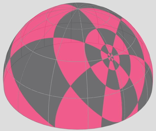
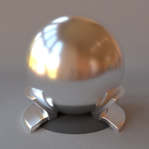
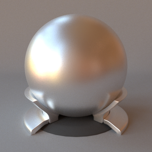
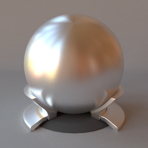
An Adaptive Parameterization for
"How to efficiently measure BRDFs with a goniophotometer"
Jonathan Dupuy
Wenzel Jakob
Unity Technologies
EPFL
This presentation is an overview of our SIGGRAPH Asia 2018 paper
"An Adaptive Parameterization for Efficient Material Acquisition and Rendering".
57 BRDFs (10 anisotropic)
[Note: this slide is progressive. Press the left key on your keyboard each
time you read [click] to keep the text in sync with the contents of
the slide]
In this paper, we introduce a novel high quality BRDF measurement database.
We have acquired this data in such a way that it can be used it
straightforwardly and efficiently for photorealistic rendering.
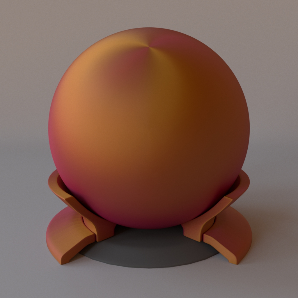
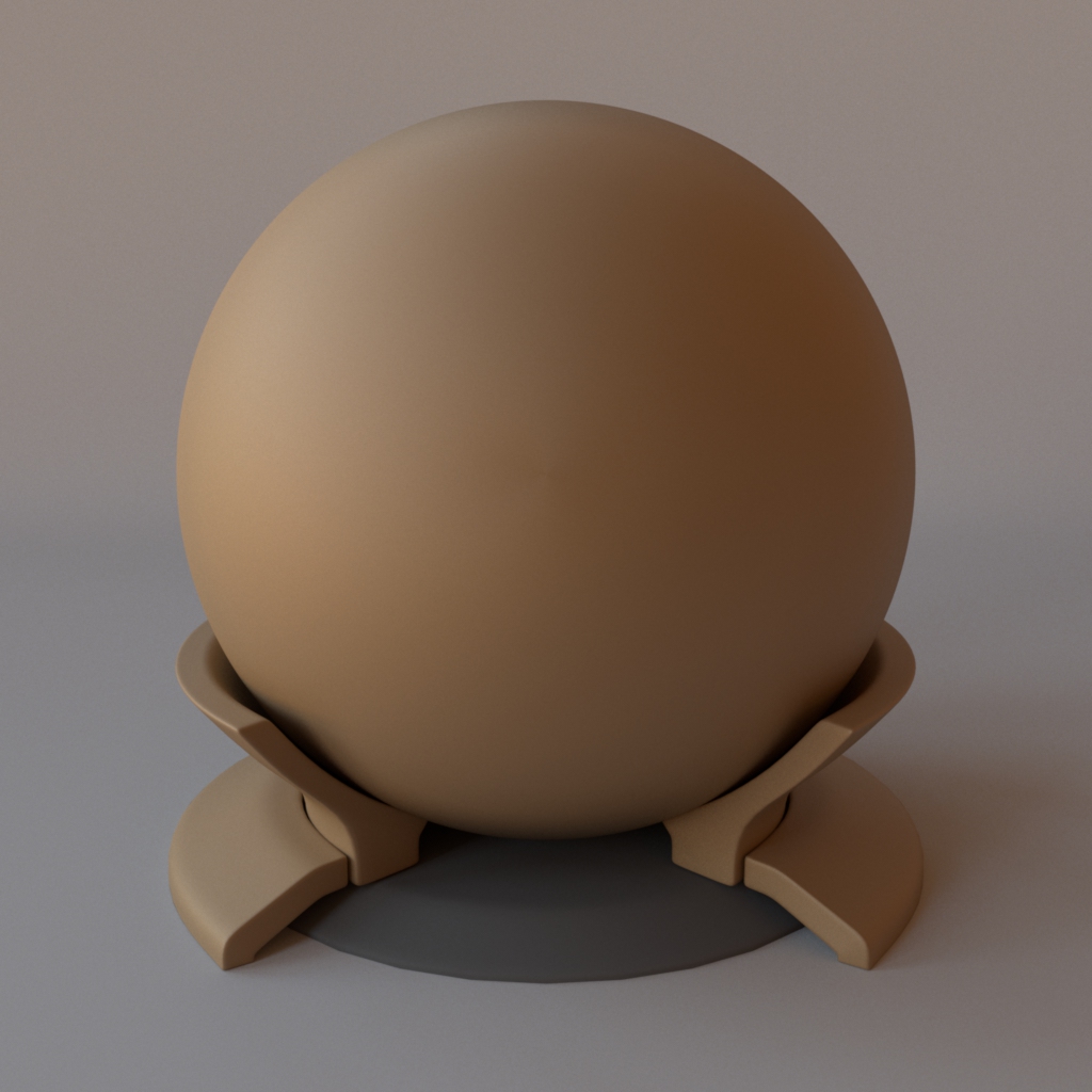
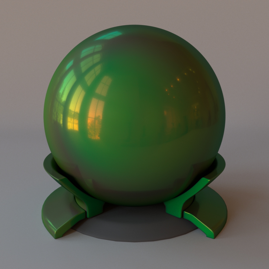
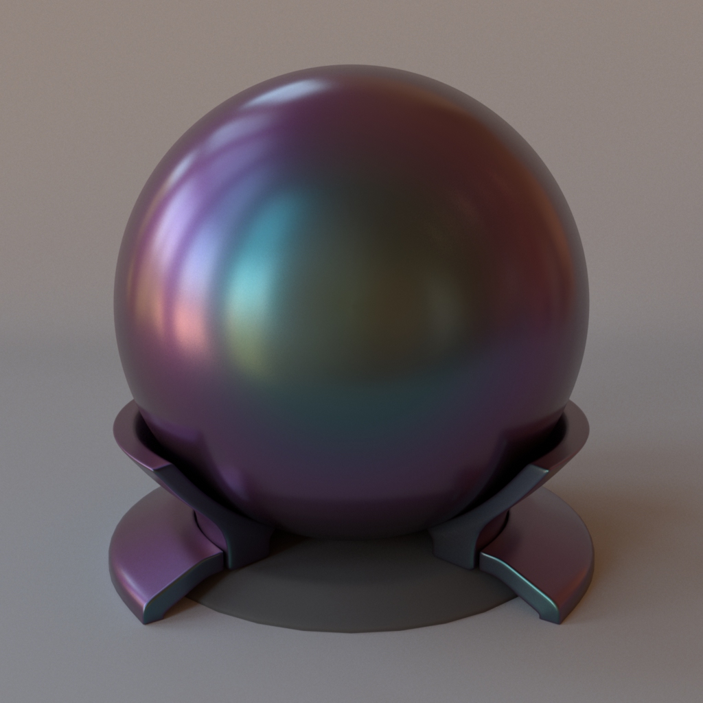
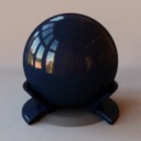
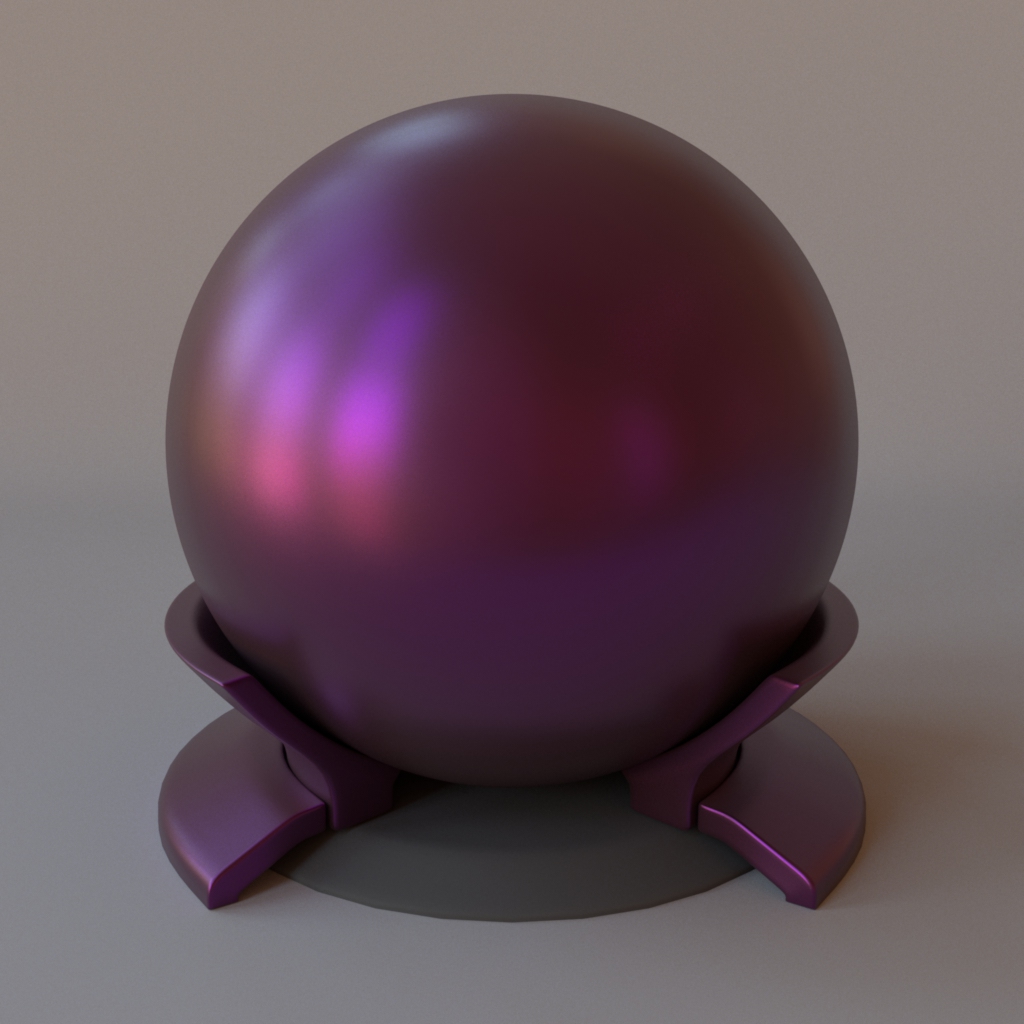
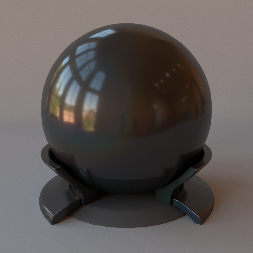
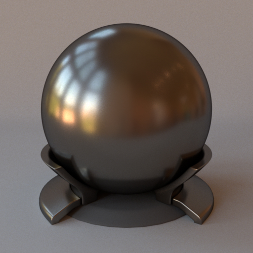
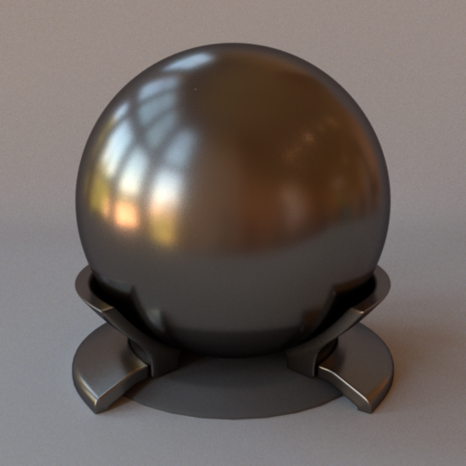
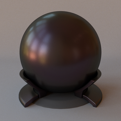
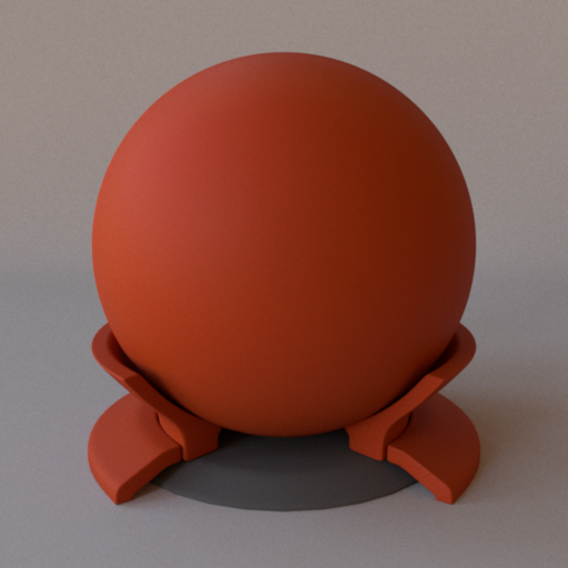
Here, we show a few such renderings, computed using 1024 samples per pixel.
Careful observers will notice
complex optical effects such as hazy gloss, opalescence, iridescence,
anisotropy, color-changing highlights, etc. Such effects are rarely seen
in computer graphics, so we're excited to have them :)
[click] 57
different materials, including 10 that exhibit highly anisotropic behaviours.
Note that this number is not fixed, as we are still growing the database with
new measurements at the present time.
Your browser does not support the video tag.
Our Pipeline
Acquisition Time:
(anisotropic) xx
2.5 days
(isotropic) xx
3 hours
[Note: this slide is progressive. Press the left key on your keyboard each
time you read [click] to keep the text in sync with the contents of
the slide]
Our measurement pipeline relies on this new theoretical framework and runs
in two steps in practice.
[click]
With our pipeline, we acquire [click] anisotropic BRDFs in 2.5 days and
[click] isotropic ones in 3 hours. We believe that such
speeds is what will make BRDF measurement feasable for photorealistic
rendering.
© Industrial Light & Magic
[Note: this slide is progressive. Press the left key on your keyboard each
time you read [click] to keep the text in sync with the contents of
the slide]
Here is a cool fact to back up this claim: when we got our first
measurements, we were discussing with ILM (Industrial Light and Magic) to
see if they could send us some of the material samples they use for the
movies they work on. It turned out that, as they were very interested in
our project, they sent us some legit Star Wars samples :)
[click] some of the materials used to build some parts of
it, which are also available for free in our database.
Motivation
Real character
Digital double
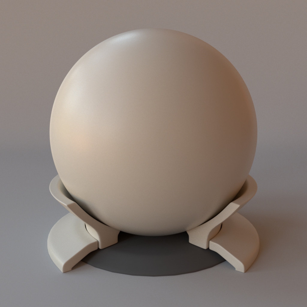
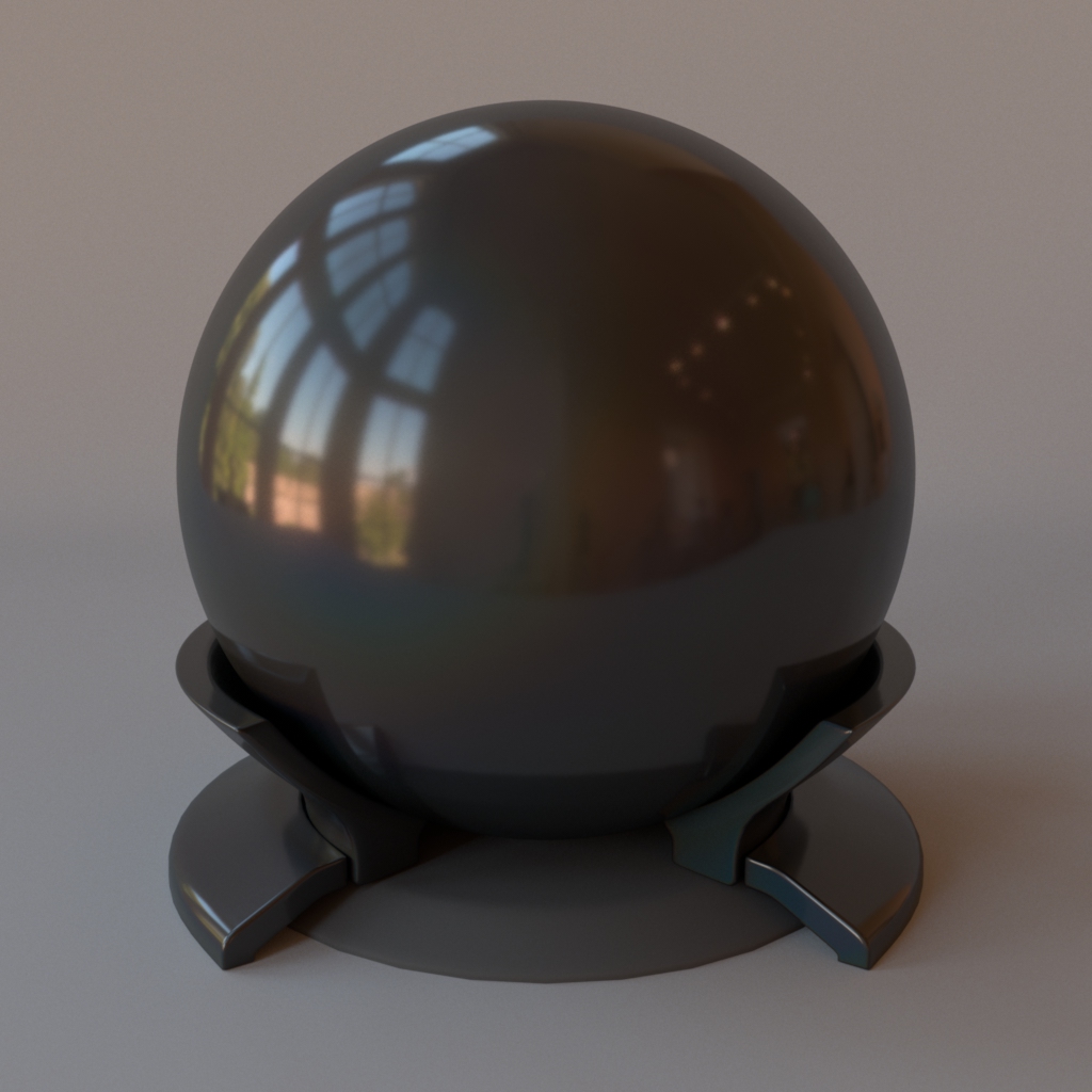
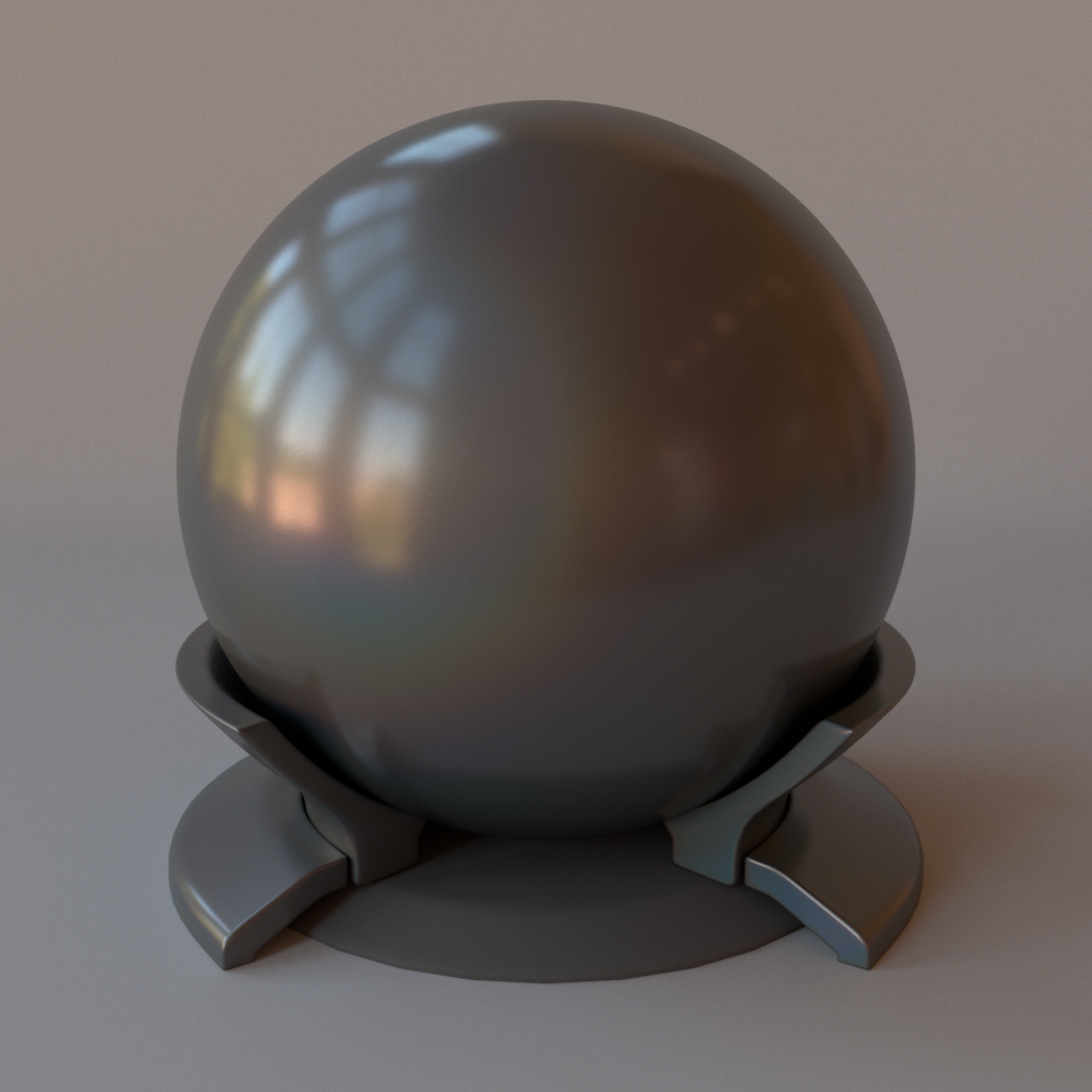
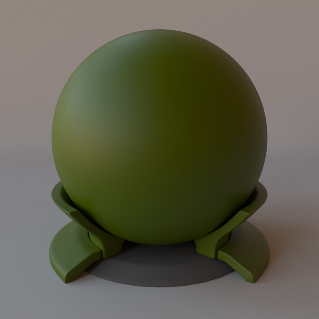
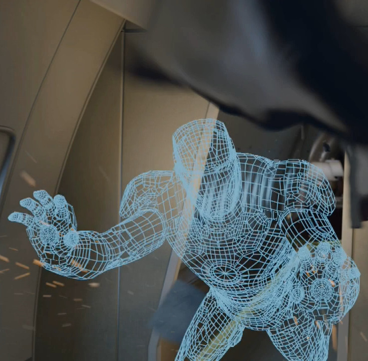
The L3-37 droid is actually a digital double. It was created from the
performance of an actress
(Phoebe Waller-Bridge, shown on the left) who was wearing a costume built so
as to carry parts of the final droid character (shown on the right).
Motivation
Real character
Digital double
Solve $$L_o = \int_{\mathcal{S}^2} L_i \cdot f_r^\perp \cdot d\boldsymbol{\omega}_i $$
[Note: this slide is progressive. Press the left key on your keyboard each
time you read [click] to keep the text in sync with the contents of
the slide]
Since ILM relies on photorealistic rendering for their special effects,
they create their digital doubles in two steps.
[click] the rendering equation, which is responsible
for giving the final photorealistic appearance to digital doubles.
Motivation
Real character
Digital double
Solve $$L_o = \int_{\mathcal{S}^2} L_i \cdot {\color{red}f_r^\perp} \cdot d\boldsymbol{\omega}_i $$
In the context of this Star Wars movie, the lighting is known beforehand.
Hence the only variable that drives the appearance of the digital double is
the term $f_r^\perp$, i.e., is the BRDF. The BRDF is responsible for
describing the way materials interact with light, and thus varies for
each material.
$$f_r^\perp = f_r(\boldsymbol{\omega}_i, \boldsymbol{\omega}_o, \lambda) \cos \theta_i$$
Incident domain
Outgoing domain
[Note: this slide is progressive. Press the left key on your keyboard each
time you read [click] to keep the text in sync with the contents of
the slide]
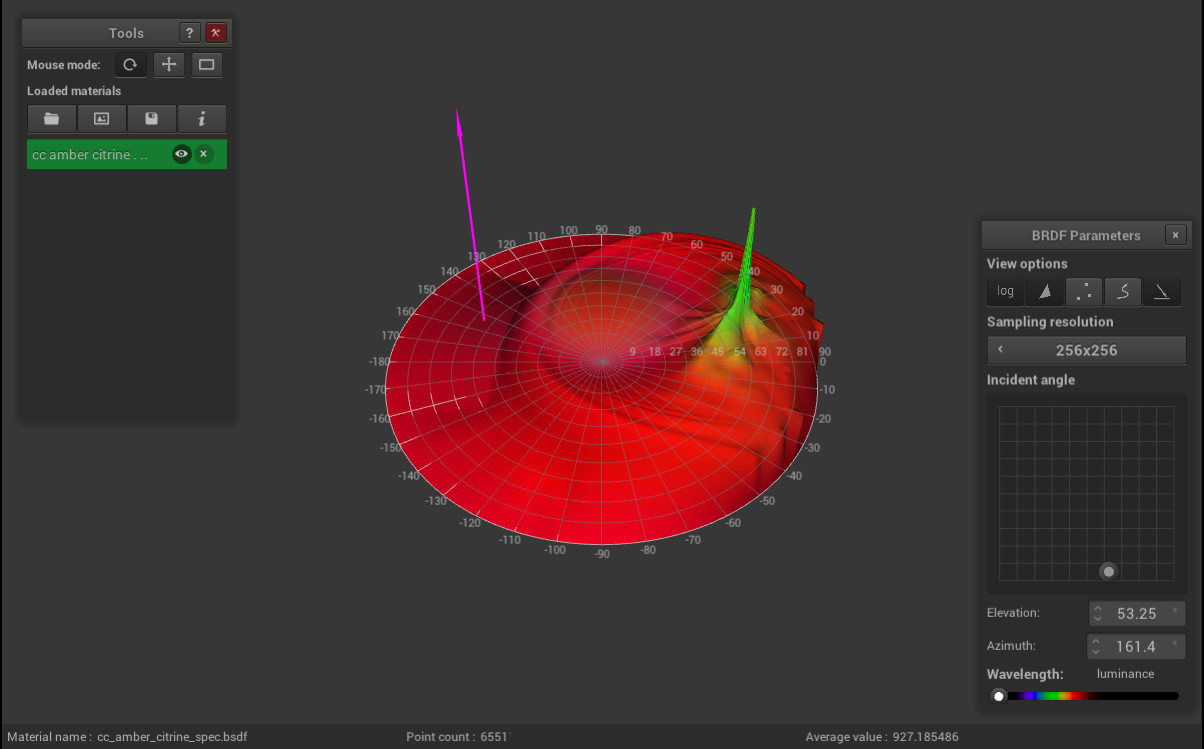
Here is an intuitive definition of the BRDF.
[click] a fixed incident direction, the BRDF describes how a
material scatters light for any [click] outgoing direction.
$$f_r^\perp = f_r(\boldsymbol{\omega}_i, \boldsymbol{\omega}_o, \lambda) \cos \theta_i$$
Your browser does not support the video tag.
Your browser does not support the video tag.
Incident domain
Outgoing domain
Wavelength
(varying)
[Note: this slide is progressive. Press the left key on your keyboard each
time you read [click] to keep the text in sync with the contents of
the slide]
Note that the shape of these BRDF lobes also vary depending on the direction
of incident light, as well as [click] on the wavelength of this
particular incident light.
Motivation
Real character
Digital double
Solve $$L_o = \int_{\mathcal{S}^2} L_i \cdot {\color{red}f_r^\perp} \cdot d\boldsymbol{\omega}_i $$
Acquire ? $$f_r^\perp = f_r^\perp(\boldsymbol{\omega}_i, \boldsymbol{\omega}_o, \lambda) $$
[Note: this slide is progressive. Press the left key on your keyboard each
time you read [click] to keep the text in sync with the contents of
the slide]
Given this definition, it is tempting to rely on [click] a
goniophotometer to actually measure how each material reacts to incident
lighting and simply use these measurements to solve the rendering equation.
Unfortunately, this was not possible until now, because such measurements
carried intractable difficulties that we will identify shortly.
Outline
What makes BRDF measurements difficult ?
A: Curse of dimensionality
How to lower the number of measurements ?
A: Image-based setup ? Use an adaptive parameterization
Is there a way to quickly characterize a material ?
A: We measure retro-reflection
Implementation details + results
Discussion
[Note: this slide is progressive. Press the left key on your keyboard each
time you read [click] to keep the text in sync with the contents of
the slide]
So why are such measurements so difficult ? In the remainder of this
presentation, we will see why and then [click] answer a series of
other questions that both describes the way we approached this problem,
and the ideas we introduce in the paper.
Problem
Incident domain
Outgoing domain
Wavelength
(2D)
(2D)
(1D)
The process of BRDF acquisition consists in exploring the high dimensional
manifold subtended by the definition of the BRDF...
Problem
Incident domain
Outgoing domain
Wavelength
(2D)
(2D)
(1D)
... and sampling each dimension so as to create a discrete version of it.
Problem
Incident domain
Outgoing domain
Wavelength
(2D)
(2D)
(1D)
✔
[Note: this slide is progressive. Press the left key on your keyboard each
time you read [click] to keep the text in sync with the contents of
the slide]
So really, this dimension is [click] not a problem in practice.
Outline
What makes BRDF measurements difficult ?
A: Curse of dimensionality
How to lower the number of measurements ?
A: Through BRDF Parameterization
Is there a way to quickly characterize a material ?
A: We look at retro-reflection
Implementation details + results
Results
[Note: this slide is progressive. Press the left key on your keyboard each
time you read [click] to keep the text in sync with the contents of
the slide]
Now, having [click] identified this issue, our only hope in making
acquisition practical is to attenuate the effects of the curse of
dimensionality. How to do such a thing ?
[click] BRDF parameterization as a
means to drastically reduce the number of measurements.
BRDF Parameterization
Incident domain
Outgoing domain
Outgoing domain
(parametric space)
[Note: this slide is progressive. Press the left key on your keyboard each
time you read [click] to keep the text in sync with the contents of
the slide]
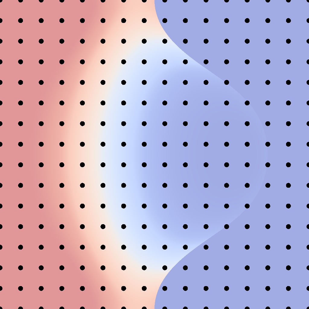
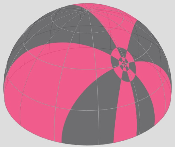
Intuitively, a parameterization is a way to look at a complex
object from a simpler one, typically a hypercube. For instance, a
parameterization of a BRDF's outgoing domain allows to visualize its
lobe inside [click] a square.
BRDF Parameterization
Incident domain
Outgoing domain
Outgoing domain
(parametric space)
Sample count:
> 2x max frequency
[Note: this slide is progressive. Press the left key on your keyboard each
time you read [click] to keep the text in sync with the contents of
the slide]
The good thing about parametric space is that it gives us a bound for the
number of measurements we need to make. Specifically, the Nyquist limit tells
that we should sample parametric space at more than twice the highest frequency
of the lobe as seen from that space.
Rusinkiewicz [1998]
Incident domain
Outgoing domain
Outgoing domain
(parametric space)
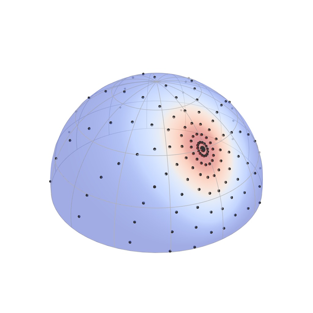
The Rusinkiewicz parameterization is a BRDF parameterization designed to do
just that. Based on the observation that BRDFs tend to peak around
the mirror reflection of the incident direction, the parameterization
places the samples around precisely this reflected direction.
Rusinkiewicz [1998]
Your browser does not support the video tag.
Your browser does not support the video tag.
Your browser does not support the video tag.
Incident domain
Outgoing domain
Outgoing domain
(parametric space)
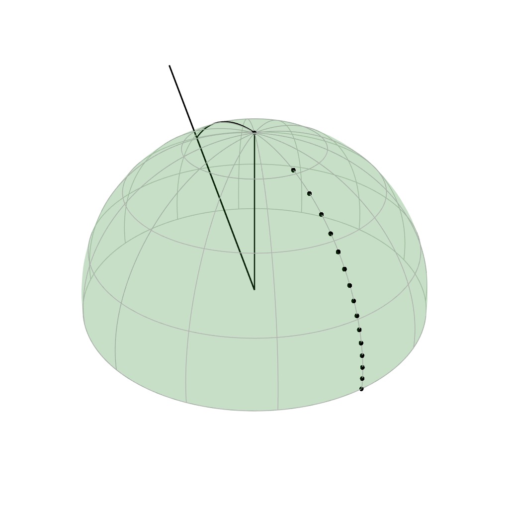
Here is an animation that shows how the samples vary as the incident
direction changes. Notice how the samples are always concentrated around
the mirror reflection of the incident direction.
MERL [Matusik et al. 2003]
Incident domain
Outgoing domain
Outgoing domain
(parametric space)
Despite these limitations, the Rusinkiewicz parameterization was
used to create the MERL database, which, up until now, was the only
all-frequency BRDF database publicly available.
MERL [Matusik et al. 2003]
Incident domain
Outgoing domain
Outgoing domain
(parametric space)
Because the Rusinkiewicz parameterization is far from perfect, it still
incurs quite a lot of measurements. To further lower this constraint,
the azimuthal dimension of incident directions was dropped. This is
acceptable if the materials under measurement are isotropic, i.e.,
they carry a radial symmetry.
Isotropic BRDFs
Your browser does not support the video tag.
Your browser does not support the video tag.
Incident domain
Outgoing domain
Outgoing domain
(parametric space)
(azimuthal symmetry)
Such a symmetry is illustrated in this animation. Notice how the shape of the
BRDF lobe is invariant to azimuthal rotation of the incident direction.
MERL [Matusik et al. 2003]
Incident domain
Outgoing domain
Outgoing domain
(parametric space)
90x90x180 resolution:
xx
16 days
x
[1 meas/s]
12 MiB
per wavelength
[Note: this slide is progressive. Press the left key on your keyboard each
time you read [click] to keep the text in sync with the contents of
the slide]
Under these assumptions, each material of the MERL database was acquired
at [click] 90x90x180 resolution, which corresponds to 1,458,000
measurements.
[click] 16 days,
which is already much better than 3+ years, but still too much to
be really practical (hence the orange color).
MERL [Matusik et al. 2003]
Spherical samples
Image-based setup
90x90x180 resolution:
xx
3 hours
x
[135 meas/s]
12 MiB
per wavelength
[Note: this slide is progressive. Press the left key on your keyboard each
time you read [click] to keep the text in sync with the contents of
the slide]
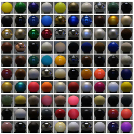
Because 16 days was still too much, Matusik et al. had a very clever idea
to further reduce these acquisition times.
[click] spherical samples, and then
built a custom [click] acquisition device based on a camera that would
take pictures of the spheres under different lighting conditions. By taking
pictures of spheres, they cover a large portion of the directional domain at
once, which strongly reduces acquisition times.
[click] 3
hours for one material, which is a huge improvement!
Outline
What makes BRDF measurements difficult ?
A: Curse of dimensionality
How to lower the number of measurements ?
Is there a way to quickly characterize a material ?
A: We look at retro-reflection
Implementation details + results
Results
[Note: this slide is progressive. Press the left key on your keyboard each
time you read [click] to keep the text in sync with the contents of
the slide]
Given such speed-ups, one may be tempted to actually follow such a setup.
Could such [click] image-based setups be the solution to BRDF acquisition ?
It turns out that this is not the case.
MERL [Matusik et al. 2003]
Spherical samples
Image-based setup
Fundamental limitations
Isotropic BRDFs only
Recquires spherical samples
Artifacts due to camera
[Note: this slide is progressive. Press the left key on your keyboard each
time you read [click] to keep the text in sync with the contents of
the slide]
The reason is because the MERL setup, while extremely fast, carries a
number of fundamental limitations.
[click]
isotropic materials. While such materials cover a wide range of real-world
materials, anisotropy is also important for e.g., fabrics or brushed metals.
[click] samples, which
are actually quite hard to manufacture and hence procure.
[click] artifacts, such as lens flare effects.
MERL [Matusik et al. 2003]
Spherical samples
Image-based setup
Fundamental limitations
Isotropic BRDFs only
Recquires spherical samples
Artifacts due to camera
source: [Lucat et al. 2017]
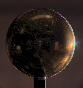
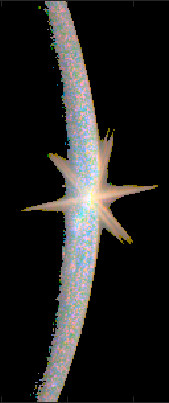
Here is an example of such an artifact. Note that this image is taken from a
recent work by Lucat et al. aiming at reproducing the setup of
Matusik et al. who were also directly confronted to these difficulties.
MERL [Matusik et al. 2003]
$\,$
$\,$
$\,$
$\,$
$\,$
$\,$
The MERL database is known to carry artifacts that can manifest in renderings
such those shown here. Notice the color-oscillations or the silver-lining
effects at grazing angles present on these MERL materials.
Outline
What makes BRDF measurements difficult ?
A: Curse of dimensionality
How to lower the number of measurements ?
Is there a way to quickly characterize a material ?
A: We look at retro-reflection
Implementation details + results
Results
So rather than relying on an image-based setup ...
Outline
What makes BRDF measurements difficult ?
A: Curse of dimensionality
How to lower the number of measurements ?
Is there a way to quickly characterize a material ?
A: We look at retro-reflection
Implementation details + results
Results
..., we decided to revisit the
parameterization. We took a step back and had a deeper analysis of the Rusinkiewicz
parameterization.
Rusinkiewicz [1998]
Your browser does not support the video tag.
Your browser does not support the video tag.
Incident domain
Outgoing domain
Outgoing domain
(parametric space)
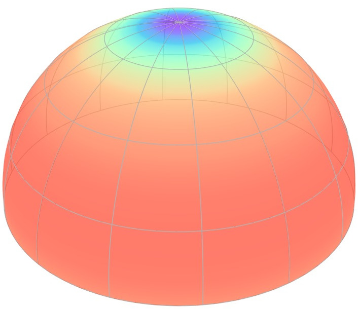
Limitation: frequency 🔗 shininess
It turns out that the Rusinkiewicz parameterization works fairly well for
rough materials, but its efficiency decreases along with shininess.
Our Approach
Your browser does not support the video tag.
Your browser does not support the video tag.
Incident domain
Outgoing domain
Outgoing domain
(parametric space)
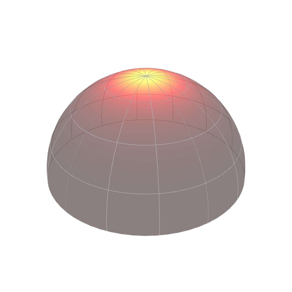
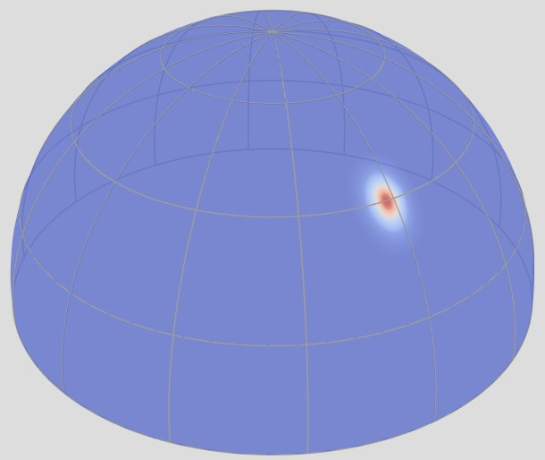
Now, since shiny materials tend to concentrate around the specular direction,
a simple way to resolve this limitation is to concentrate the parameterization
near the mirror-reflection direction. This animation shows just that.
Outline
What makes BRDF measurements difficult ?
A: Curse of dimensionality
How to lower the number of measurements ?
A: Image-based setup ? Use an adaptive parameterization
Is there a way to quickly characterize a material ?
A: We measure retro-reflection
Implementation details + results
Results
[Note: this slide is progressive. Press the left key on your keyboard each
time you read [click] to keep the text in sync with the contents of
the slide]
This is the fundamental idea behind our paper: develop an [click]
adaptive parameterization based on the shininess of the material we want to
measure.
[click] the retro-reflection domain of the BRDF.
Retro-reflective Domain (2D)
$f_r^\perp(\boldsymbol{\omega}_i = \boldsymbol{\omega}_o)$
Rough
Shiny
Anisotropic
45x180 resolution:
xx
2 hours
x
[1 meas/s]
31 KiB
per wavelength
[Note: this slide is progressive. Press the left key on your keyboard each
time you read [click] to keep the text in sync with the contents of
the slide]
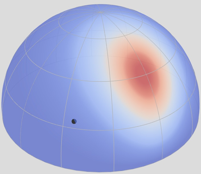
The retro-reflective domain is the directional sub-domain of the BRDF that
corresponds to the configurations where [click] the incident and
outgoing directions are aligned, i.e., $\boldsymbol{\omega}_i = \boldsymbol{\omega}_o$.
[click] shiny materials
have a narrow retro-reflective lobes, [click] rough materials have wide
ones, and finally [click] anistropic materials exhibit a radial
asymmetry.
[click] it is both fast to acquire,
and easy to store.
Retro-reflective Domain (2D)
$f_r^\perp(\boldsymbol{\omega}_i = \boldsymbol{\omega}_o)$
Rough
Shiny
Anisotropic
Now, these properties are quite straightforward in retrospect, but
of course we did not find them by chance ;)
Why Retro-reflection ?
${\color{red}f_r^\perp}(\boldsymbol{\omega}_i = \boldsymbol{\omega}_o)$
Actually, there is a theoretical justification to why we build our
parameterization using retro-reflection. This justification is microfacet
theory.
Microfacet Theory
${\color{red}f_r^\perp}(\boldsymbol{\omega}_i = \boldsymbol{\omega}_o)$
[Note: this slide is progressive. Press the left key on your keyboard each
time you read [click] to keep the text in sync with the contents of
the slide]
Microfacet theory is a theoretical framework that justifies the behaviours
of BRDFs by modelling them as [click] the global response of a
collection of microscropic mirrors.
Microfacet Theory
NDF
${\color{red}f_r^\perp}(\boldsymbol{\omega}_i = \boldsymbol{\omega}_o)$
NDF: ${\color{blue}D}(\boldsymbol{\omega}_m)$
This particular description is provided by the microfacet normal
distribution unction (NDF), which tells how much mirror (micro)area is
oriented towards a specific direction.
Microfacet Theory
NDF
${\color{red}f_r^\perp}(\boldsymbol{\omega}_i = \boldsymbol{\omega}_o)$
NDF: ${\color{blue}D}(\boldsymbol{\omega}_m)$
intuition:
$
{\color{red}f_r^\perp}(\boldsymbol{\omega}_i, \boldsymbol{\omega}_o)
\propto
{\color{blue}D}(\boldsymbol{\omega}_h)
$
The reason why the NDF plays an important role in microfacet theory is
this.
Retro-reflection
NDF
${\color{red}f_r^\perp}(\boldsymbol{\omega}_i = \boldsymbol{\omega}_o)$
NDF: ${\color{blue}D}(\boldsymbol{\omega}_m)$
intuition:
$
{\color{red}f_r^\perp}(\boldsymbol{\omega}_i = \boldsymbol{\omega}_o)
\propto
{\color{blue}D}(\boldsymbol{\omega}_h)
$
Under this assumption, it follows that under retro-reflective configurations,
the amount of energy should be directly proportional to the value of the NDF.
Retro-reflection
NDF
${\color{red}f_r^\perp}(\boldsymbol{\omega}_i = \boldsymbol{\omega}_o)$
NDF: ${\color{blue}D}(\boldsymbol{\omega}_m)$
intuition:
$
{\color{red}f_r^\perp}(\boldsymbol{\omega}_i = \boldsymbol{\omega}_o)
\propto
{\color{blue}D}(\boldsymbol{\omega}_h)
$
This suggests that we can retrieve a microfacet NDF from an arbitrary material
solely from its retro-reflection responses.
NDF Extraction
NDF
${\color{red}f_r^\perp}(\boldsymbol{\omega}_i = \boldsymbol{\omega}_o)$
NDF: ${\color{blue}D}(\boldsymbol{\omega}_m)$
Solve Fredholm equation of the second kind
with Kernel
$$
K(\boldsymbol{\omega}, \boldsymbol{\omega}_m)
=
{\color{red}f_r^\perp}(\boldsymbol{\omega}, \boldsymbol{\omega})
\langle
\boldsymbol{\omega}
\cdot
\boldsymbol{\omega}_m
\rangle
$$
intuition:
$
{\color{red}f_r^\perp}(\boldsymbol{\omega}_i = \boldsymbol{\omega}_o)
\propto
{\color{blue}D}(\boldsymbol{\omega}_h)
$
Actually in the paper, we show that this relation writes down to a simple equation
that relates the NDF (written in blue) to [click] the retro-reflection
response of the material (written in red).
[click] a Fredholm equation of
the second kind and we explain how to solve it in an efficient and robust
way using power iterations over an eigenvector problem. More details are in
the paper.
Retro-reflection Acquisition
NDF
${\color{red}f_r^\perp}(\boldsymbol{\omega}_i = \boldsymbol{\omega}_o)$
NDF: ${\color{blue}D}(\boldsymbol{\omega}_m)$
intuition:
$
{\color{red}f_r^\perp}(\boldsymbol{\omega}_i = \boldsymbol{\omega}_o)
\propto
{\color{blue}D}(\boldsymbol{\omega}_h)
$
laser
beam dump
photodiode
beamsplitter
sample
isolator
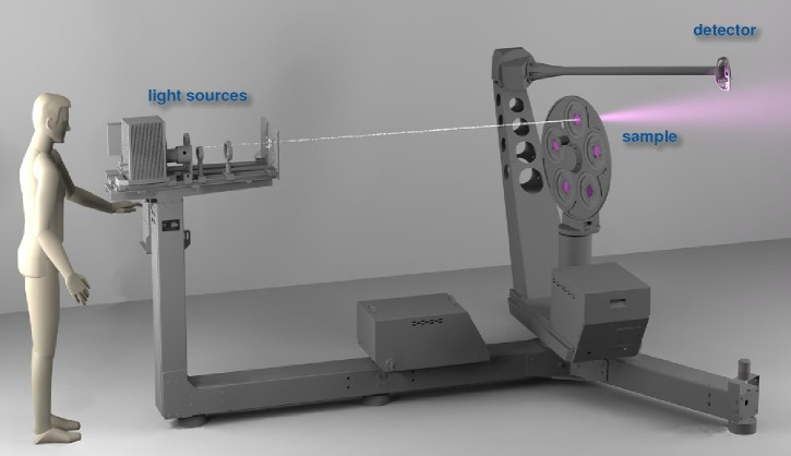
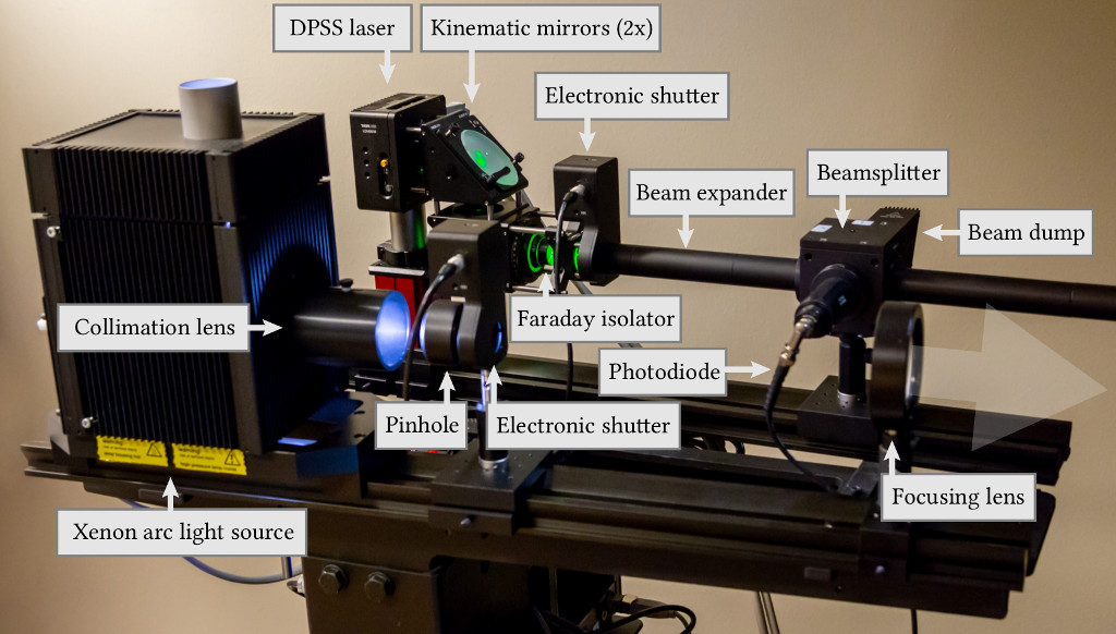
Note that acquiring retro-reflection can be quite tricky in practice and we
have a specific setup solely dedicated to that purpose. The setup is based on
a laser and a beam splitter that partially lets the light through to
illuminate the sample and reflects some of the scattered light into a
photodiode. More details are in the paper.
Our Parameterization
NDF
NDF: ${\color{blue}D}(\boldsymbol{\omega}_m)$
Once we have extracted a microfacet NDF from the material we wish to acquire
we then proceed to build our adaptive parameterization that we leverage to
perform 4D measurements at low resolution.
Our Parameterization
NDF
NDF: ${\color{blue}D}(\boldsymbol{\omega}_m)$
Here again, our parameterization is based on insights from microfacet theory.
Our Parameterization
NDF
NDF: ${\color{blue}D}(\boldsymbol{\omega}_m)$
$\boldsymbol{\omega}_m$
$\boldsymbol{\omega}_i$
Specifically, we rely on the notion of projected areas of the microfacets...
Our Parameterization
NDF
NDF: ${\color{blue}D}(\boldsymbol{\omega}_m)$
$\boldsymbol{\omega}_m$
$\boldsymbol{\omega}_i$
$\langle
\boldsymbol{\omega}_i
\cdot
\boldsymbol{\omega}_m
\rangle$
..., which are directly subject to the cosine attenuation law, or Lambert's
attenuation law.
Our Parameterization
NDF
NDF: ${\color{blue}D}(\boldsymbol{\omega}_m)$
$\boldsymbol{\omega}_m$
$\boldsymbol{\omega}_i$
$\langle
\boldsymbol{\omega}_i
\cdot
\boldsymbol{\omega}_m
\rangle$
intuition: sample
$
\propto
\langle
\boldsymbol{\omega}_i
\cdot
\boldsymbol{\omega}_m
\rangle
{\color{blue}D}(\boldsymbol{\omega}_m)
$
Under this intuition, we devise our parameterization such that it importance
samples these projected areas.
Our Parameterization
NDF
NDF: ${\color{blue}D}(\boldsymbol{\omega}_m)$
intuition: sample
$
\propto
\langle
\boldsymbol{\omega}_i
\cdot
\boldsymbol{\omega}_m
\rangle
{\color{blue}D}(\boldsymbol{\omega}_m)
$
$\boldsymbol{\omega}_m$
$\boldsymbol{\omega}_i$
$\langle
\boldsymbol{\omega}_i
\cdot
\boldsymbol{\omega}_m
\rangle$
parametric
BRDF
$\;$
$$g$$
$$\;\;\shortmid\!\longrightarrow\;$$
.
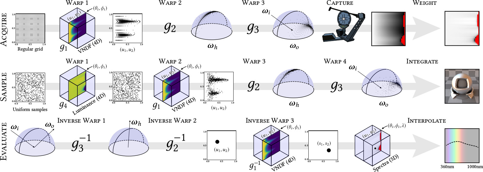
This is the foundation of our adaptive parameterization, which leverages a
bijective mapping between the BRDF's directional space and that of a
unit hypercube.
Our Parameterization
NDF
NDF: ${\color{blue}D}(\boldsymbol{\omega}_m)$
intuition: sample
$
\propto
\langle
\boldsymbol{\omega}_i
\cdot
\boldsymbol{\omega}_m
\rangle
{\color{blue}D}(\boldsymbol{\omega}_m)
$
$\boldsymbol{\omega}_m$
$\boldsymbol{\omega}_i$
$\langle
\boldsymbol{\omega}_i
\cdot
\boldsymbol{\omega}_m
\rangle$
parametric
BRDF
$\;$
$$g$$
$$\;\;\shortmid\!\longrightarrow\;$$
.
Built-in importance sampling
[Note: this slide is progressive. Press the left key on your keyboard each
time you read [click] to keep the text in sync with the contents of
the slide]
For those who are familiar with microfacet theory, this approach is based
exactly on the importance sampling mechanism of Heitz and d'Eon.
[click] an efficient importance sampling
mechanism, because the way we importance sample it is exactly the same as the
one we use to measure it in the first place.
Our Parameterization
$f_r^\perp(\boldsymbol{\omega}_i = \boldsymbol{\omega}_o)$
Incident domain
Outgoing domain
Prepass, then:
[Importance Sample]
[Importance Sample]
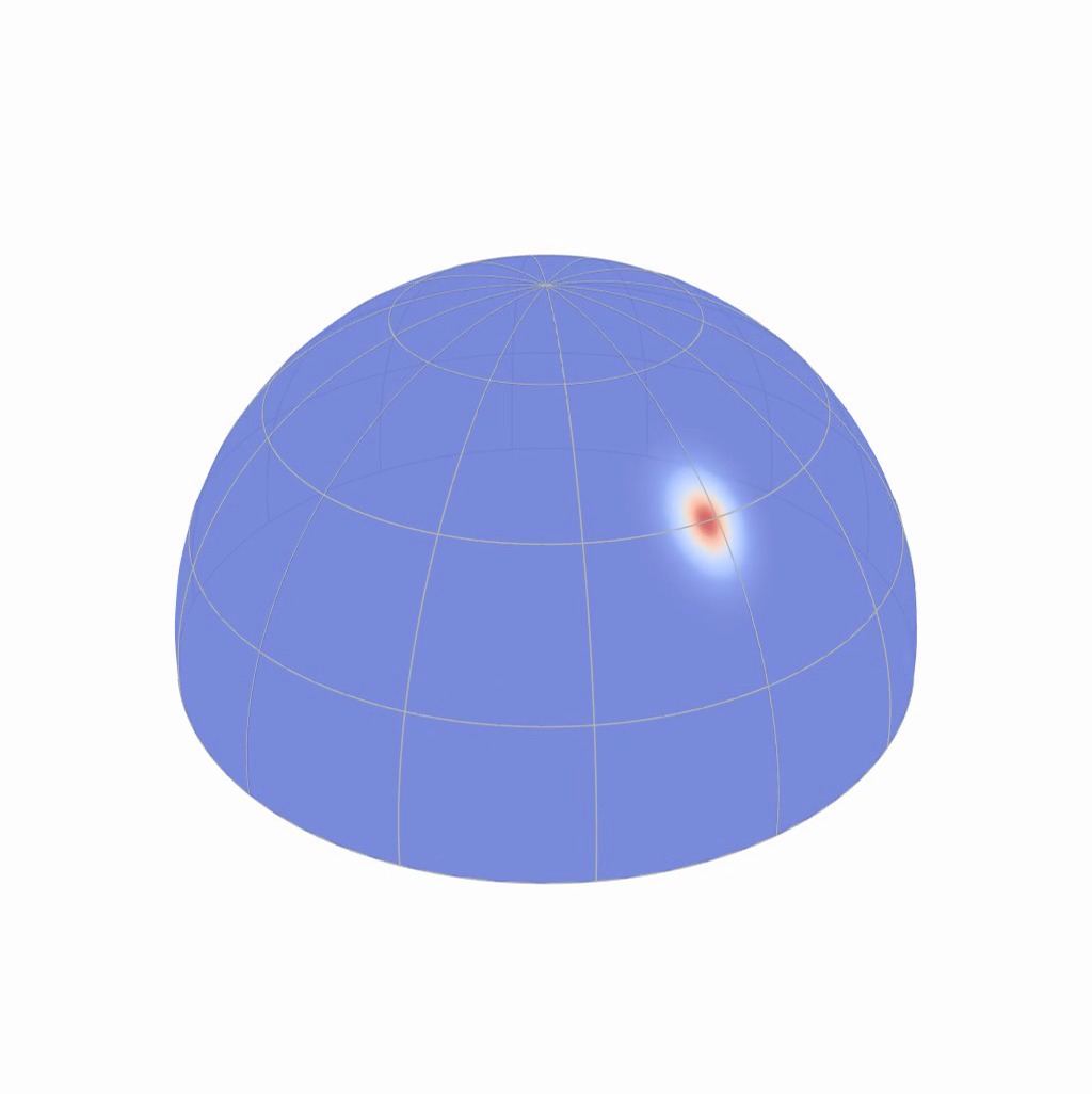
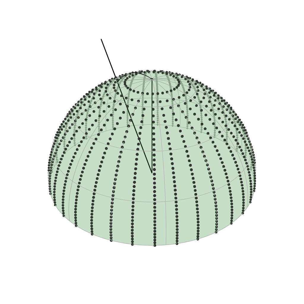
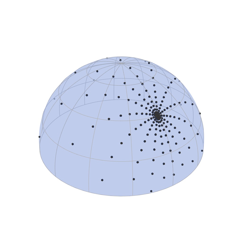
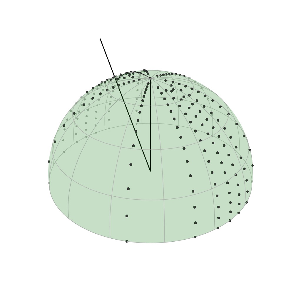
... that effectively importance samples the 4D directional domain of the BRDF.
Our Parameterization
$f_r^\perp(\boldsymbol{\omega}_i = \boldsymbol{\omega}_o)$
Incident domain
Outgoing domain
Prepass, then:
[Importance Sample]
[Importance Sample]
32x32
In practice we discretize the outgoing domain at 32x32 resolution.
Our Parameterization
$f_r^\perp(\boldsymbol{\omega}_i = \boldsymbol{\omega}_o)$
Incident domain
Outgoing domain
Shiny Material
Prepass, then:
[Importance Sample]
[Importance Sample]
32x32
As expected, the samples get more concentrated for shiny materials...
Our Parameterization
$f_r^\perp(\boldsymbol{\omega}_i = \boldsymbol{\omega}_o)$
Incident domain
Outgoing domain
Rough Material
Prepass, then:
[Importance Sample]
[Importance Sample]
32x32
... and more dilated for rough materials...
Our Parameterization
$f_r^\perp(\boldsymbol{\omega}_i = \boldsymbol{\omega}_o)$
Incident domain
Outgoing domain
Anisotropic Material
Prepass, then:
[Importance Sample]
[Importance Sample]
32x32
... If the input material is anisotropic, then the samples are warped along
the main directions of radial asymetry.
Our Parameterization
$f_r^\perp(\boldsymbol{\omega}_i = \boldsymbol{\omega}_o)$
Incident domain
Outgoing domain
Anisotropic Material
Prepass, then:
[Importance Sample]
[Importance Sample]
32x32
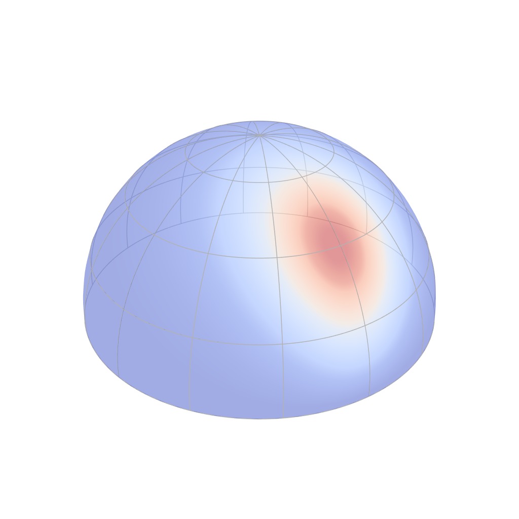
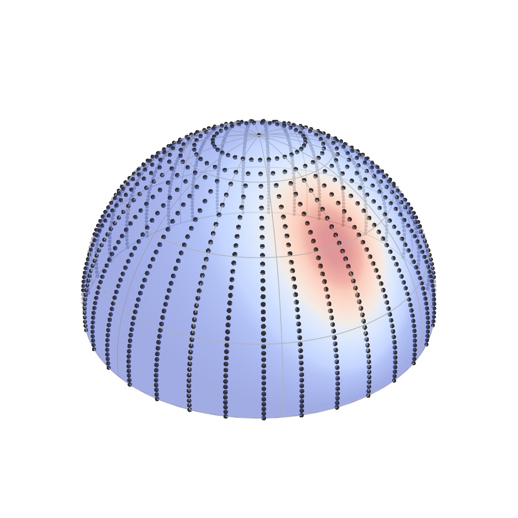
(here is the final BRDF lobe to emphasize that the samples are indeed placed
at efficient locations)
Our Parameterization
$f_r^\perp(\boldsymbol{\omega}_i = \boldsymbol{\omega}_o)$
Incident domain
Outgoing domain
Anisotropic Material
Prepass, then:
[Importance Sample]
[Importance Sample]
32x32
8x16
100K samples:
xx
2.5 days
x
[1 meas/s]
512 KiB
per wavelength
We discretize the incident domain into 8 elevations and 16 azimuthal angles,
so that their distribution also accounts for the characteristics of the
material. For instance, in the case of an anisotropic material, the azimuthal
distribution of incident samples will concentrate around the regions of
high curvature, where anisotropy leads to more dramatic BRDF variations.
[click] 2.5
days in total, recquiring a 512KiB of memory per wavelength.
Our Parameterization
$f_r^\perp(\boldsymbol{\omega}_i = \boldsymbol{\omega}_o)$
Incident domain
Outgoing domain
Anisotropic Material
Prepass, then:
[Importance Sample]
[Importance Sample]
32x32
8x16
And that's for the case of an anisotropic BRDF.
Our Parameterization
$f_r^\perp(\boldsymbol{\omega}_i = \boldsymbol{\omega}_o)$
Incident domain
Outgoing domain
Isotropic Material
Prepass, then:
[Importance Sample]
[Importance Sample]
32x32
8x1
8K samples:
xx
2.2 hours
x
[1 meas/s]
32 KiB
per wavelength
It turns out that for isotropic BRDFs, which we can detect via their
radially symmetric retro-reflective lobes, we can be even faster.
For such materials,
only a single slice of the incident domain is necessary due to radial
symmetry (just as for the MERL database).
[click] 3
hours in total, recquiring a 32KiB of memory per wavelength.
Your browser does not support the video tag.
Our Pipeline
Here is our measurement pipeline again. Showing the retro-reflective response
and the 4D measurements.
OK now let's see some cool acquisition results. Our database
is entirely free and available online at [click] the following
website [website live demo].
Results (1024 spp)
Microfacet-like
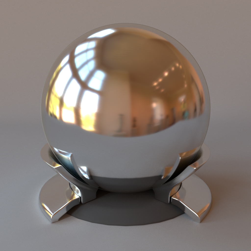
vch_dragon_eye_red
vch_frozen_amethyst
vch_silk_blue
vch_ultra_pink
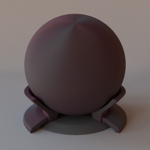
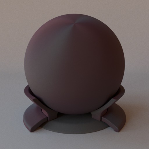
Here are a few selected materials. Such glossy highlights are typically perfect
candidates for microfacet theory.
Results (1024 spp)
Microfacet-like
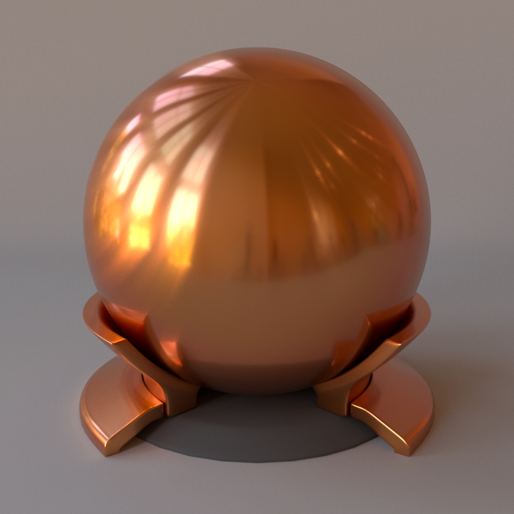
aniso_copper_sheet
aniso_metallic_paper_copper
aniso_metallic_paper_gold
aniso_brushed_aluminium
Hazy lobes
Here is another set of good candidates, altough they exhibit anisotropy and
super hazy lobes that are very difficult to model with analytic microfacet
NDFs; such materials could serve as reference for modelling new hazy NDFs.
Results (1024 spp)
Microfacet-like ?
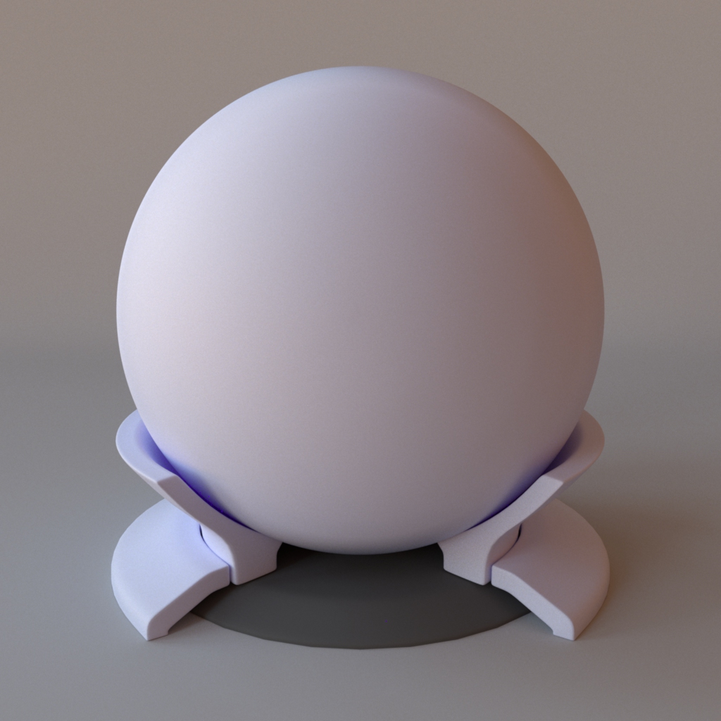
satin_white
satin_blue
satin_gold
satin_purple
Coloured-highlights
Moving on to another set of candidates, alreay more complicated as they
exhibit colored highlights that are hard to explain and/or model with
microfacet theory.
Results (1024 spp)
Microfacet-like ?
aurora_white
cc_nothern_aurora
aniso_sari_silk_2color
aniso_morpho_melenaus
Funky!
And finally a set of aliens (!). All these materials exhibit wave-optics
behaviours that are completely alien to microfacet theory, which is a
geometric optics model.
Outline
What makes BRDF measurements difficult ?
A: Curse of dimensionality
How to lower the number of measurements ?
A: Image-based setup ? Use an adaptive parameterization
Is there a way to quickly characterize a material ?
A: We measure retro-reflection
Implementation details + results
Results
Take aways:
(BRDF modelling & rendering) xx
New public spectral BRDF database
(gonio-photometric acquisition) xx
New practical acquisition technique
[Note: this slide is progressive. Press the left key on your keyboard each
time you read [click] to keep the text in sync with the contents of
the slide]
We are now reaching the end of this presentation.
As the exposition has been quite dense, here are [click] two targetted
take-aways to wrap everything up.
[click] First, if you happen to be working on BRDF modelling or
photorealistic rendering, then there is a new spectral database
available online to download.
[click] Second, if you happen to own a BRDF acquisition device, then
there is a new efficient algorithm you can rely on to build your own database.
Acknowledgements
Naty Hoffman (ILM) Andre Mazzone (ILM) Olesya Jakob
Benoit Ruiz
Peter Apian-Bennewitz
Laurent Belcour
Romain Pacanowski
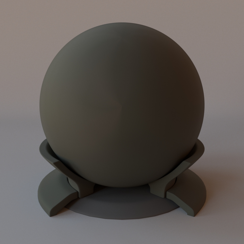
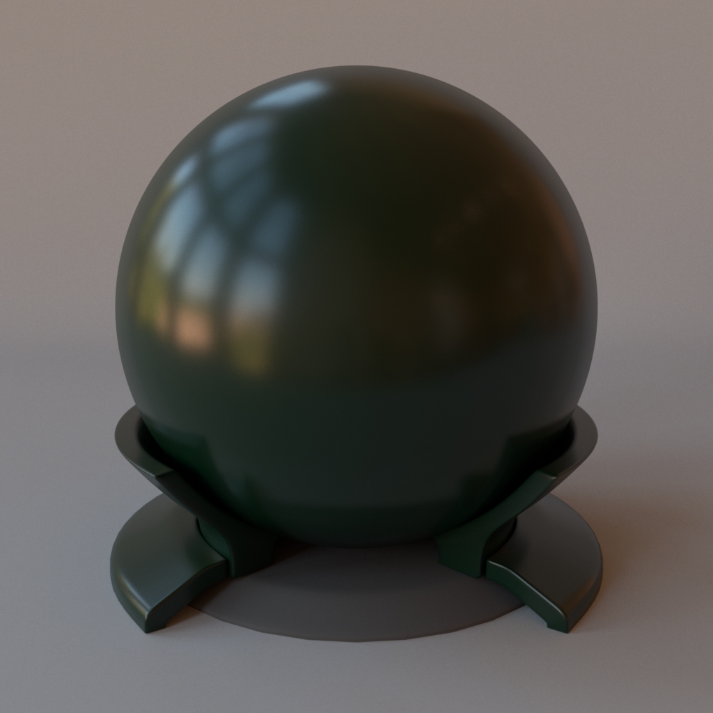
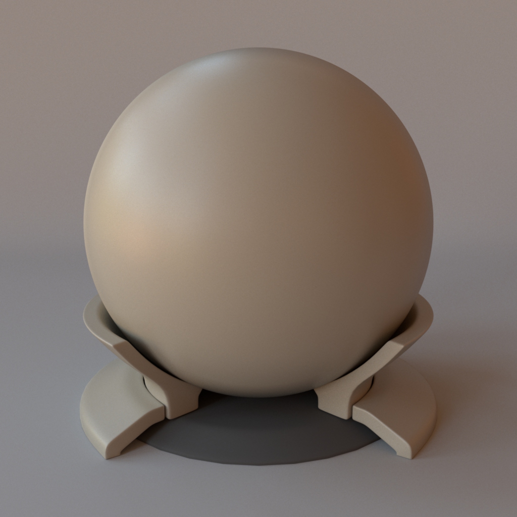
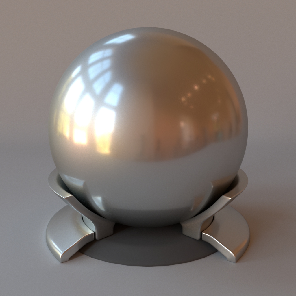
darth_vader_pants
millennium_falcon
tarkin_tunic
solo_m_68
Industrial ? Your material here !
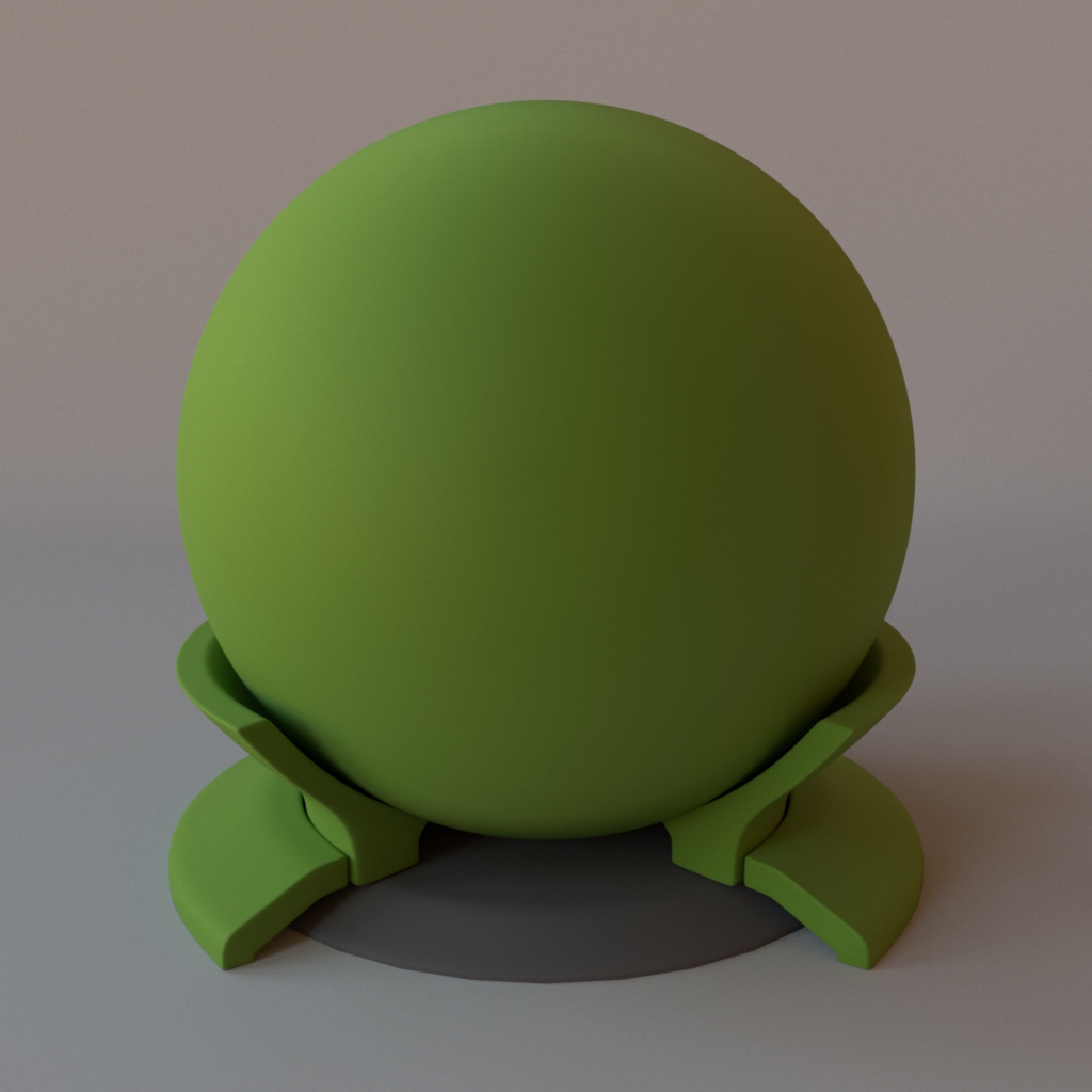
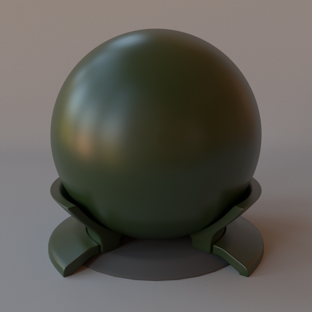
l3_37_dark_green
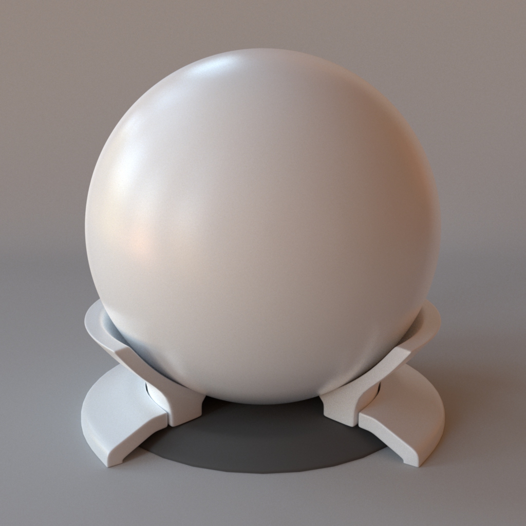
l3_37_matte
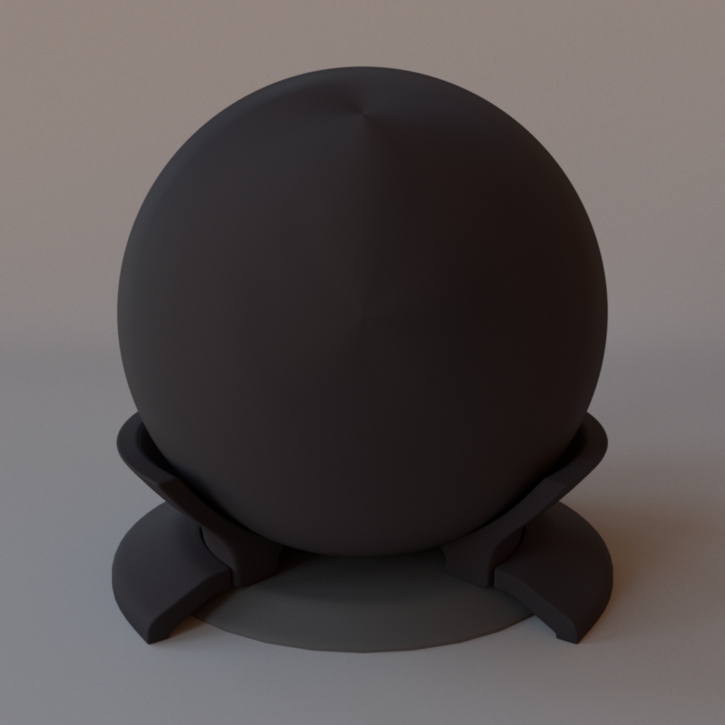
l3_37_metallic
Many thanks to Naty Hoffman and Andre Mazzone from ILM to have provided
us with the Star Wars materials.
Acknowledgements
Naty Hoffman (ILM)
Andre Mazzone (ILM)
Olesya Jakob Benoit Ruiz
Peter Apian-Bennewitz
Laurent Belcour
Romain Pacanowski
Olesya Jakob created this nice 3D scene that we used in our paper.
Acknowledgements
Naty Hoffman (ILM)
Andre Mazzone (ILM)
Olesya Jakob Benoit Ruiz
Peter Apian-Bennewitz
Laurent Belcour
Romain Pacanowski
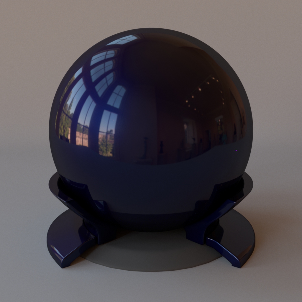
Since our acquisitions are spectral, we played with the spectra of the light
sources in the scene. Notice how the materials can take very different
appearances depending on the lighting conditions. This is an area we have not
explored in detail, but believe it to be important as it widens the
range of expressiveness wrt traditional RGB rendering.
Acknowledgements
Naty Hoffman (ILM)
Andre Mazzone (ILM)
Olesya Jakob
Benoit Ruiz Peter Apian-Bennewitz
Laurent Belcour
Romain Pacanowski
Thanks to Benoit Ruiz, a student from EPFL, who implemented the
BRDF viewer that's available online.
Acknowledgements
Naty Hoffman (ILM)
Andre Mazzone (ILM)
Olesya Jakob
Benoit Ruiz
Peter Apian-Bennewitz Laurent Belcour
Romain Pacanowski
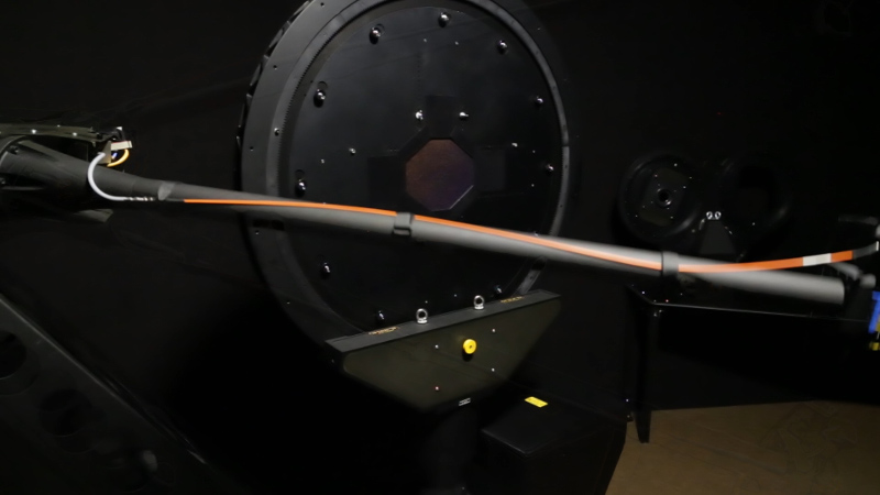
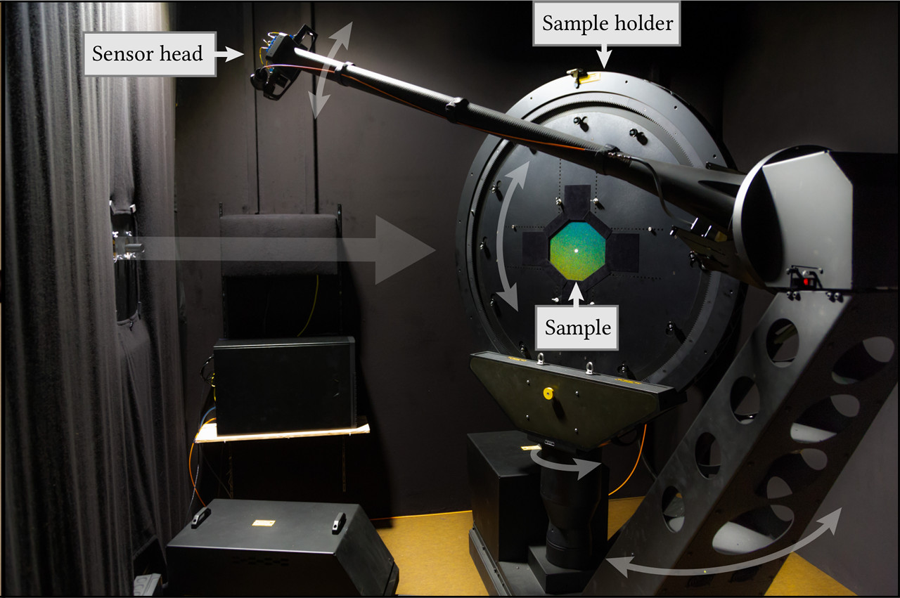
Thanks to Peter Apian-Bennewitz who is the builder of the goniophotometer
we used to perform our measurements and provided us with software support.
Acknowledgements
Naty Hoffman (ILM)
Andre Mazzone (ILM)
Olesya Jakob
Benoit Ruiz
Peter Apian-Bennewitz
Laurent Belcour Romain Pacanowski
laser
beam dump
photodiode
beamsplitter
sample
isolator
Finally, thanks to Laurent Belcour and Romain Pacanowski for sharing their
insights on how to measure retro-reflection using a beam splitter.
This is the end of the talk. Here is the URL that will take you to the
database. Enjoy !
Storage
$\;\;\;$
$\;\;\;$
$\;\;\;$
$\;\;\;$
$\;\;\;$
$\;\;\;$
Storage
$\;\;\;$
$\;\;\;$
$\;\;\;$
$\;\;\;$
$\;\;\;$
$\;\;\;$
Validation: MERL
Ref (36 MiB)
Ours (96 KiB)
Ref (36 MiB)
Ours (96 KiB)
Importance Sampling
$$L_o = \int_{\mathcal{H}^2} L_i \cdot f_r^\perp \cdot d\boldsymbol{\omega}_i$$
In a rendering context, we use importance sampling of the BRDF x cos.
It turns out that this is exactly what we would like to do for a material.
But measured materials don't have builtin importance sampling. So we looked
into microfacet theory. Microfacet theory is a mathematical framework that
has undergone a large evolution due to CG and has been successful at
explaining the behaviour of real world materials and has a good importance
sampling mechanism.
We could devise an importance sampling mechanism for any BRDF, but only
if we know it before hand, which means we need to measure it !
So we simplify the problem to acquiring a microfacet BRDF.
So we decided to simplify our acquisition paper into that of acquiring
a microfacet BRDF.
The equation itself is not very interesting.
Microfacet theory describes the behaviour of
materials as a collection of flakes and blabla, NDF.
Given an NDF, we can build an importance sampling mechanism that consists
in picking a microfacet proportionally visible area; this is called the VNDF
sampling.
Importance Sampling
$$L_o = \int_{\mathcal{H}^2} L_i \cdot f_r^\perp \cdot d\boldsymbol{\omega}_i$$
Substitution
$$\boldsymbol{\omega}_i = g(\mathbf{u})$$
$$
\Rightarrow d\boldsymbol{\omega}_i = \left| \frac{dg}{d\mathbf{u}} \right| d\mathbf{u}
$$
$$= \int_{\mathcal{U}^2} L_i \cdot f_r^\perp \cdot \left| \frac{dg}{d\mathbf{u}} \right| \cdot d\mathbf{u}$$
parametric domain
BRDF domain
$$g$$ $$\shortmid\!\longrightarrow$$ .
$$\;\;\;\; g^{-1}$$ $$\longleftarrow\!\shortmid$$ .
Importance Sampling
$$L_o = \int_{\mathcal{H}^2} L_i \cdot f_r^\perp \cdot d\boldsymbol{\omega}_i$$
$$= \int_{\mathcal{U}^2} L_i \cdot f_r^\perp \cdot \left| \frac{dg}{d\mathbf{u}} \right| \cdot d\mathbf{u}$$
Substitution
$$\boldsymbol{\omega}_i = g(\mathbf{u})$$
$$
\Rightarrow d\boldsymbol{\omega}_i = \left| \frac{dg}{d\mathbf{u}} \right| d\mathbf{u}
$$
parametric domain
BRDF domain
$$g$$ $$\shortmid\!\longrightarrow$$ .
$$\;\;\;\; g^{-1}$$ $$\longleftarrow\!\shortmid$$ .
low-frequency
Perfect sampling condition:
$$ \left| \frac{dg}{d\mathbf{u}} \right| \propto \frac{1}{f_r^\perp}$$
$$f_r^\perp \cdot \left| \frac{dg}{d\mathbf{u}} \right|$$
In a rendering context, we use importance sampling of the BRDF x cos.
It turns out that this is exactly what we would like to do for a material.
But measured materials don't have builtin importance sampling. So we looked
into microfacet theory. Microfacet theory is a mathematical framework that
has undergone a large evolution due to CG and has been successful at
explaining the behaviour of real world materials and has a good importance
sampling mechanism.
We could devise an importance sampling mechanism for any BRDF, but only
if we know it before hand, which means we need to measure it !
So we simplify the problem to acquiring a microfacet BRDF.
So we decided to simplify our acquisition paper into that of acquiring
a microfacet BRDF.
The equation itself is not very interesting.
Microfacet theory describes the behaviour of
materials as a collection of flakes and blabla, NDF.
Given an NDF, we can build an importance sampling mechanism that consists
in picking a microfacet proportionally visible area; this is called the VNDF
sampling.
Importance Sampling
$$L_o = \int_{\mathcal{H}^2} L_i \cdot f_r^\perp \cdot d\boldsymbol{\omega}_i$$
$$= \int_{\mathcal{U}^2} L_i \cdot f_r^\perp \cdot \left| \frac{dg}{d\mathbf{u}} \right| \cdot d\mathbf{u}$$
Substitution
$$\boldsymbol{\omega}_i = g(\mathbf{u})$$
$$
\Rightarrow d\boldsymbol{\omega}_i = \left| \frac{dg}{d\mathbf{u}} \right| d\mathbf{u}
$$
parametric domain
BRDF domain
$$g$$ $$\shortmid\!\longrightarrow$$ .
$$\;\;\;\; g^{-1}$$ $$\longleftarrow\!\shortmid$$ .
low-frequency
Perfect sampling condition:
$$ \left| \frac{dg}{d\mathbf{u}} \right| \propto \frac{1}{f_r^\perp}$$
$$f_r^\perp \cdot \left| \frac{dg}{d\mathbf{u}} \right|$$
Importance sampling
Parameterization
Efficient importance sampling
$\Rightarrow$
Adaptive parameterization
In a rendering context, we use importance sampling of the BRDF x cos.
It turns out that this is exactly what we would like to do for a material.
But measured materials don't have builtin importance sampling. So we looked
into microfacet theory. Microfacet theory is a mathematical framework that
has undergone a large evolution due to CG and has been successful at
explaining the behaviour of real world materials and has a good importance
sampling mechanism.
We could devise an importance sampling mechanism for any BRDF, but only
if we know it before hand, which means we need to measure it !
So we simplify the problem to acquiring a microfacet BRDF.
So we decided to simplify our acquisition paper into that of acquiring
a microfacet BRDF.
The equation itself is not very interesting.
Microfacet theory describes the behaviour of
materials as a collection of flakes and blabla, NDF.
Given an NDF, we can build an importance sampling mechanism that consists
in picking a microfacet proportionally visible area; this is called the VNDF
sampling.
BRDF Acquisition
Gonioreflectometer setup
Pab PGII Retroreflection
BRDF domain
Practical concerns
Shadowing
Symmetries
Validation
BRDF Acquisition
Gonioreflectometer setup
Pab PGII
Retroreflection BRDF domain
Practical concerns
Shadowing
Symmetries
Validation
laser
beam dump
photodiode
beamsplitter
sample
isolator
BRDF Acquisition
Gonioreflectometer setup
Pab PGII
Retroreflection
BRDF domain
Practical concerns
Shadowing
Symmetries
Validation
xenon arc lamp
sample
sensor
collimation
lens
focusing
lens
pinhole
BRDF Acquisition
Shadowed!
$$f_r^\perp = f_r(\boldsymbol{\omega}_i, \boldsymbol{\omega}_o, \lambda) \cos \theta_i$$
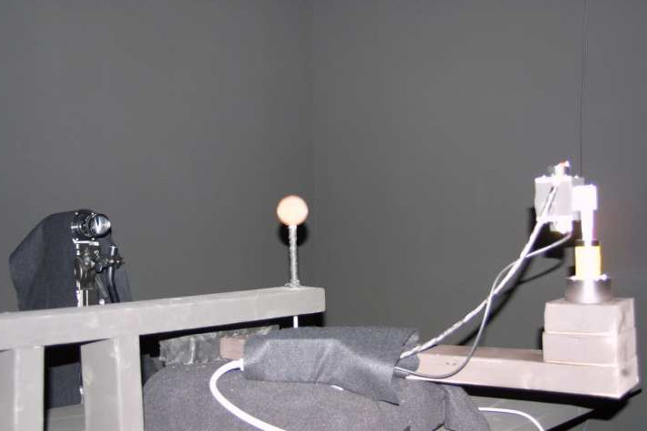
Setup for BRDF Acquisition
Overview
To this end, we introduce a novel parameterization for BRDFs.
A parameterization provides a mapping, say
$g$, that transforms a parametric domain
--typically the unit hypercube-- into a domain of interest --here
the directional domain. This mapping is invertible, meaning that
any signal on the domain of interest can be warped to the parametric
domain. In this work, we make sure that the warped signal is as low
frequency as possible. Now, there are plenty of ways to design such
parameterizations, but what makes ours special is that
Overview
There are two key features that our parameterization provides.
First, it is adaptive: it produces a smmoth signal in
the parametric domain, indepently from that of the
original signal expressed in the domain of interest.
Overview
Second, it is predictive. This means that our parameterization adapts to
the material without having full knowledge of the input signal. This is
crucial in the context of acquisition since we don't want to have to
acquire a full 5D BRDF beforehand.
